I wanted to connect the parts of torch.compile that are often explained separately. Capturing a graph is one problem. Turning it into efficient kernels is another. Reusing that work safely on the next call adds a whole set of caches and runtime checks.
This is the blog version of my end-to-end talk. Each slide has a short explanation below it, and you can click the diagrams to open the full-size image. The internal names describe the implementation explored in the talk; they aren’t a stable public API.
1. Following the whole journey

We’ll start with the Python function you write and follow it until compiled work runs on the device. The goal is to understand what each stage receives and what it produces. Once those boundaries are clear, a slow first call or an unexpected recompile becomes easier to investigate.
2. What is torch.compile?
torch.compile prepares a callable that can capture and optimize supported parts of a PyTorch program. With the default Inductor backend, this can produce generated kernels and calls to existing libraries. It supports both training and inference, but it doesn’t promise that every Python statement becomes device code or that every workload gets faster.
3. The first call and later calls
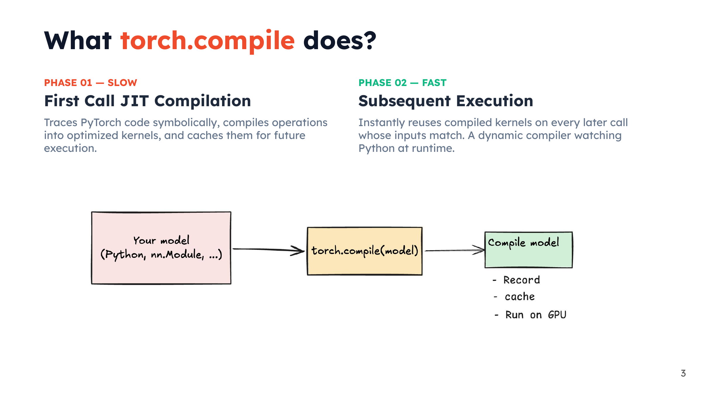
The first invocation commonly pays for tracing and compilation. Later calls can reuse compiled artifacts when the relevant assumptions still hold. There may also be warmup, autotuning, or CUDA graph capture before execution settles down. This is why measuring just one invocation tells a very incomplete performance story.
4. Where the overhead comes from
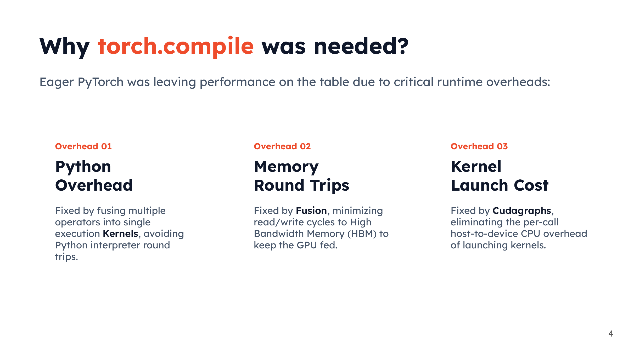
Small operations can spend a surprising amount of time in Python dispatch, intermediate memory traffic, and kernel launches. Capturing a region reduces repeated dispatch, fusion can avoid intermediate reads and writes, and CUDA graphs can reduce CPU launch overhead when enabled. These optimizations address different costs; none removes the actual computation the model needs.
5. A small vocabulary
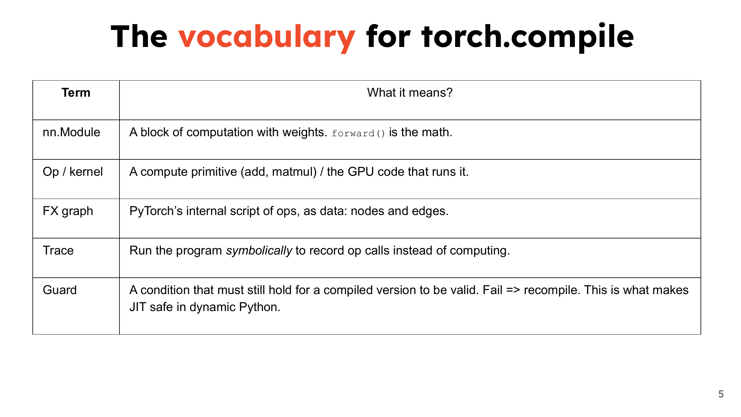
An operation describes computation, while a kernel is one implementation that executes it. An FX graph records operations and their dependencies. A guard checks an assumption needed to reuse a compiled result. One failed guard doesn’t always mean immediate compilation: another cached version may still match.
6. The main stages
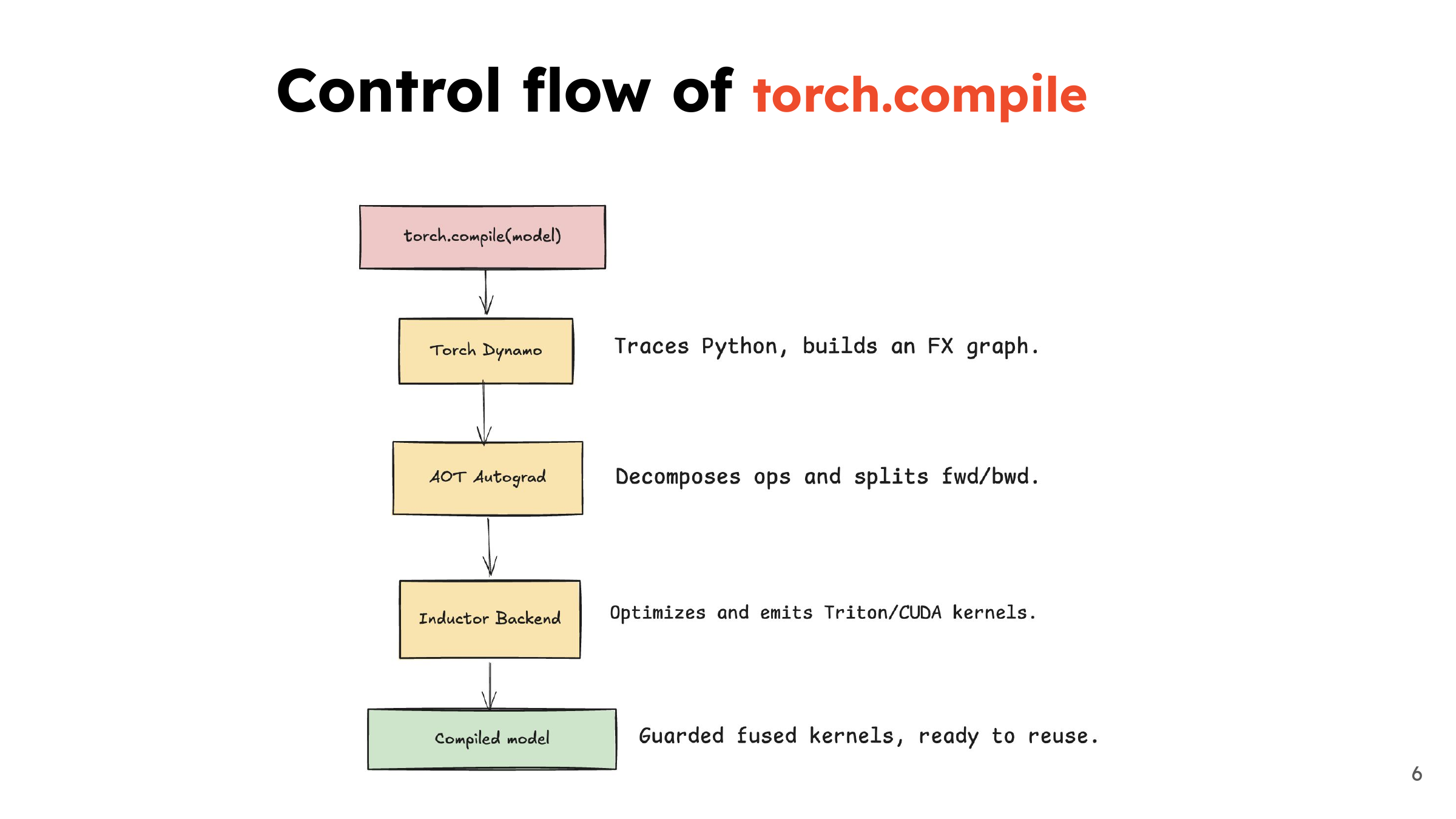
Dynamo captures Python execution into FX graphs. AOTAutograd handles transformations such as functionalization and, for training, preparing forward and backward graphs. Inductor lowers the resulting computation, schedules it, and generates executable code. Each stage works at a different level of detail, which is why the intermediate representations keep changing.
7. Reading the complete map
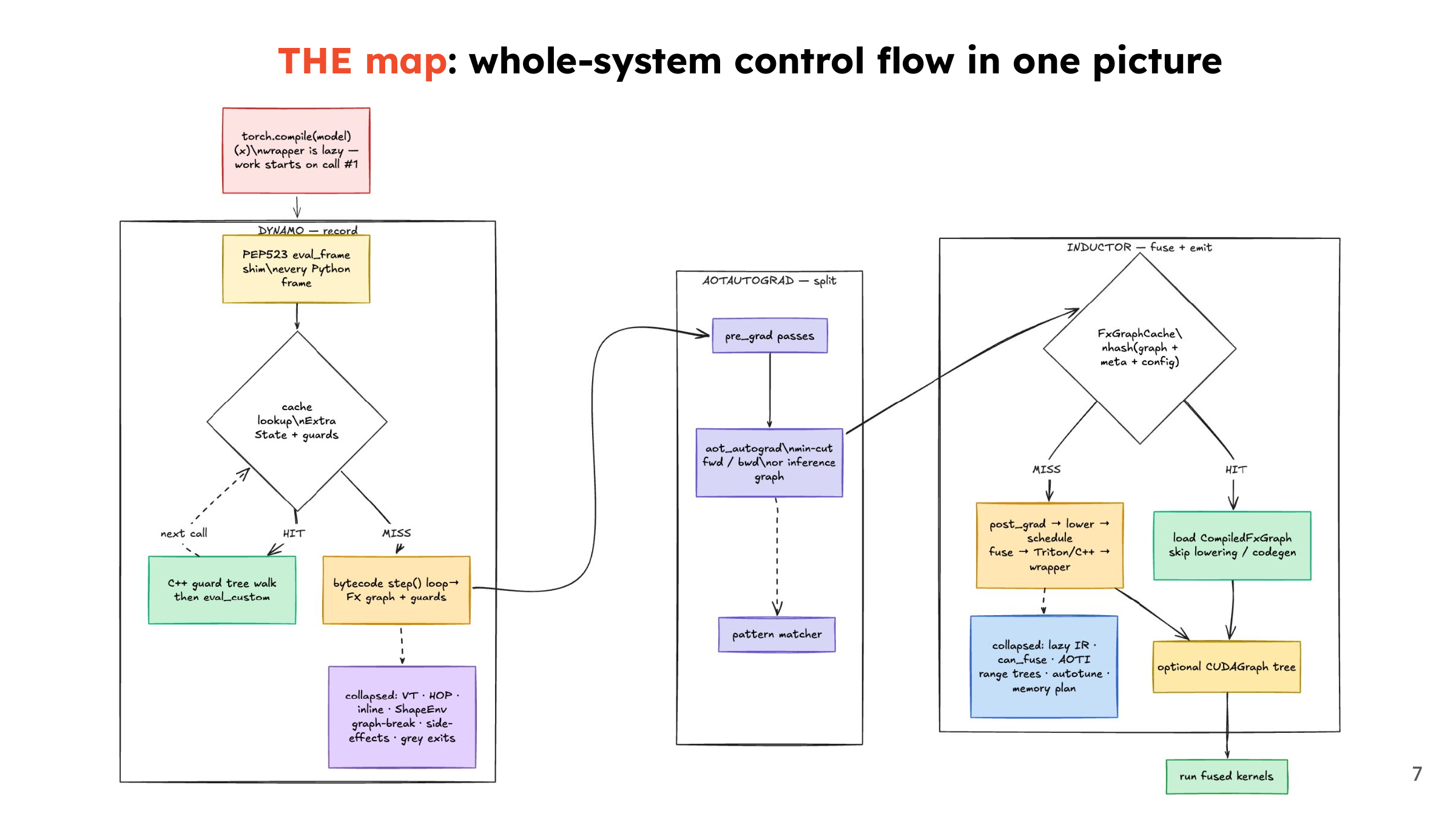
The large diagram includes the return paths that a simple pipeline picture leaves out. Cache hits can skip expensive work, guards can send execution back toward tracing, and CUDA graph replay has its own conditions. I find it helpful to follow one first call all the way through before looking at the shorter reuse paths.
8. A cache miss versus a cache hit
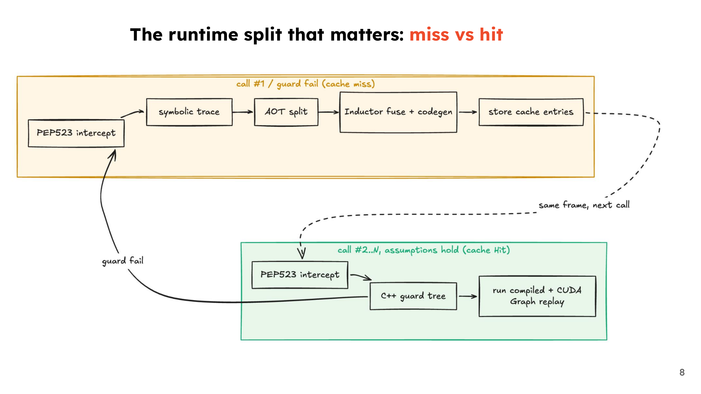
On a miss, the system may trace, transform, compile, and store a new result. On a hit, it checks the relevant guards and dispatches to work that already exists. A fresh Dynamo trace can still hit a lower compiler cache, so a miss at one layer doesn’t necessarily mean every layer starts from scratch.
9. Dynamo’s responsibilities
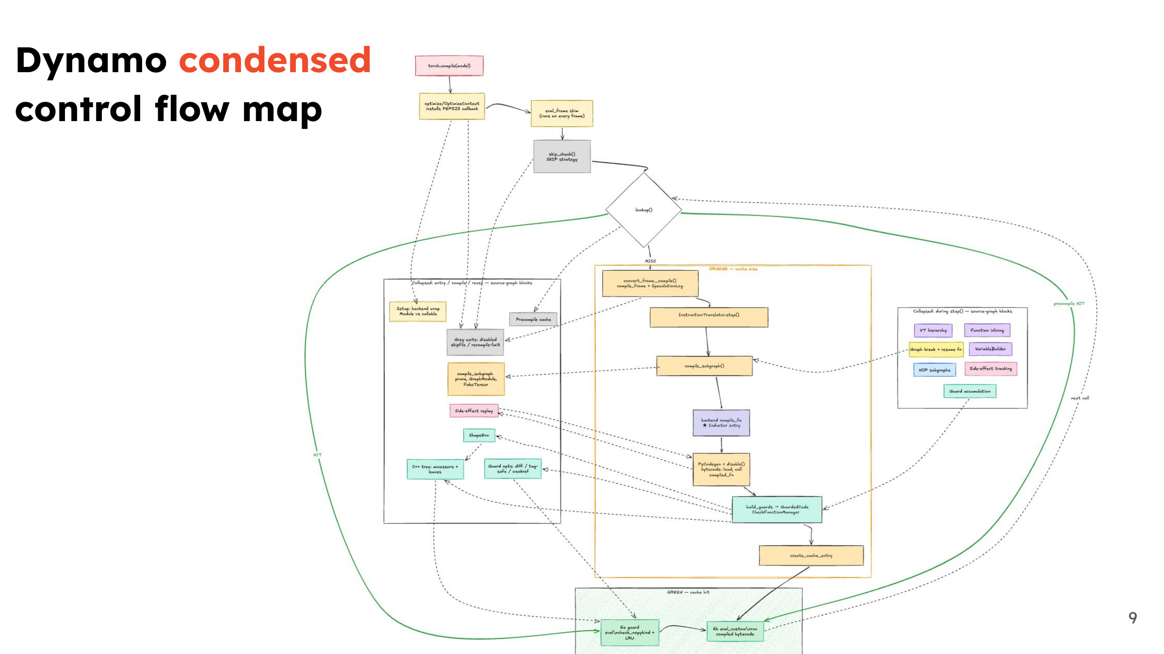
Dynamo has to understand Python values well enough to capture tensor operations without changing program behavior. Alongside graph construction, it tracks assumptions and supported side effects. The output combines graph calls with residual Python execution. This explains why Dynamo’s implementation contains much more than a recorder for torch operations.
10. Frame evaluation and lookup
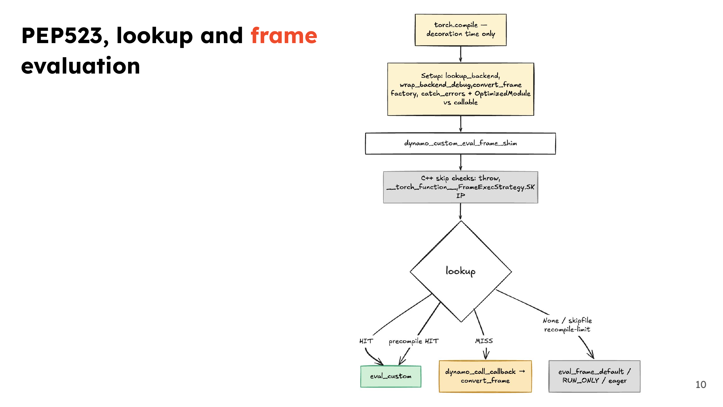
The frame evaluation hook is where execution enters Dynamo’s runtime machinery. It can find a matching cached result, invoke tracing, or allow ordinary Python execution depending on the frame and configuration. The frame evaluator source is useful for following those choices.
11. Inside step()
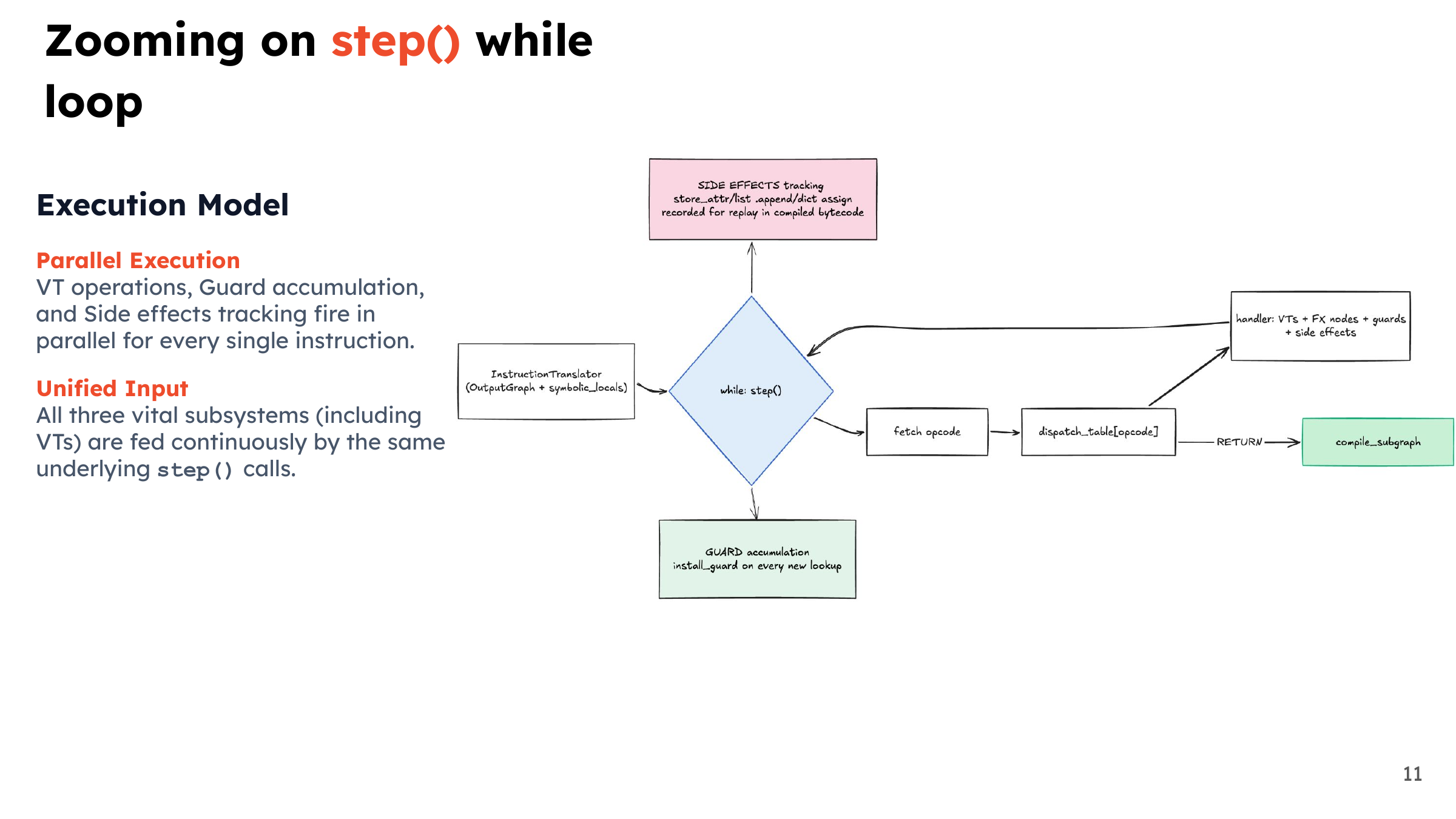
step() processes an instruction through the symbolic interpreter’s dispatch table. Value tracking, guard creation, and side-effect tracking develop together as instructions are handled. The slide calls this parallel execution, but these are cooperating responsibilities in the tracing process; it doesn’t mean three worker threads run for every bytecode instruction.
12. Three outputs from one trace
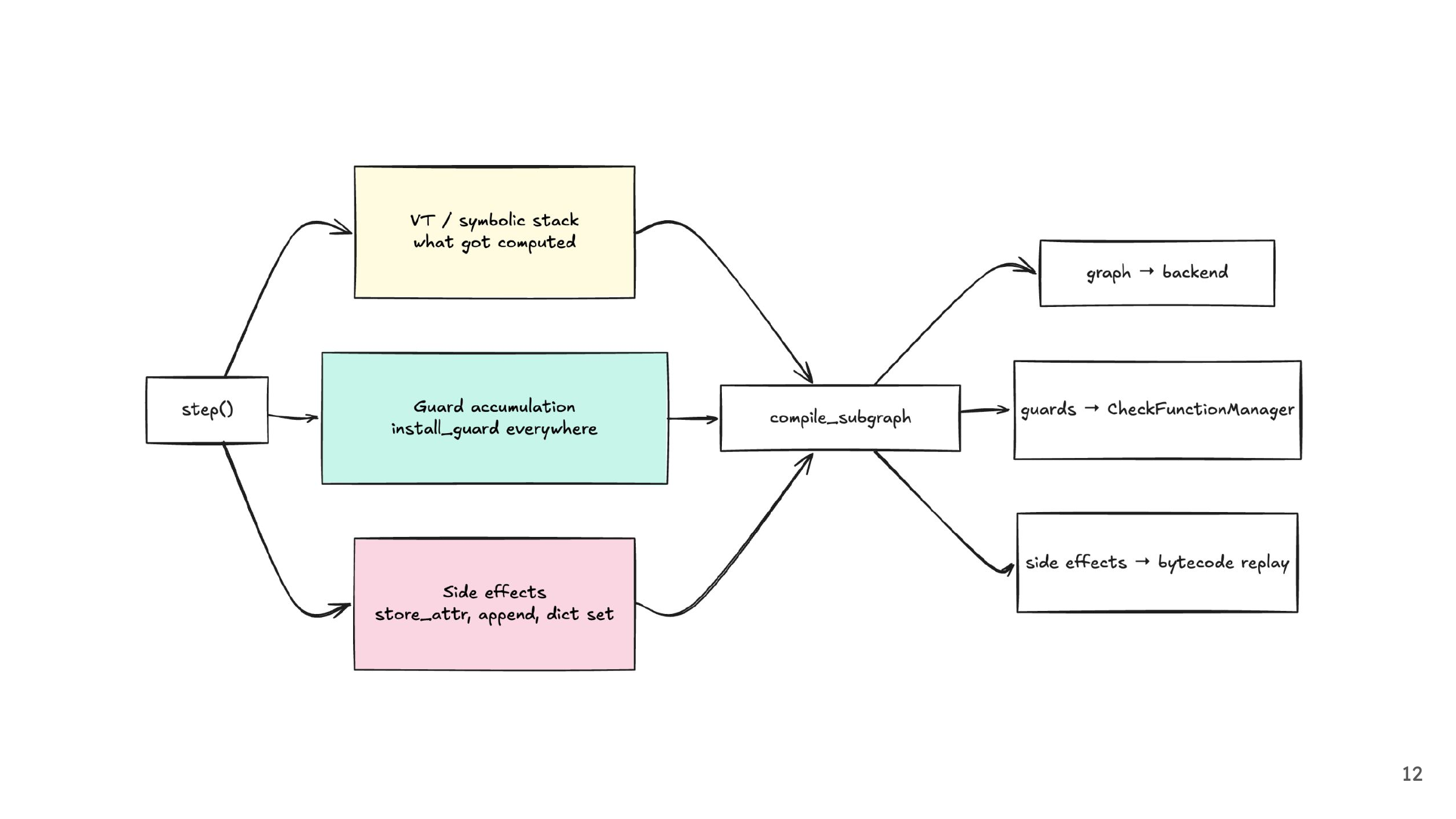
The graph describes tensor computation, guards describe when reuse is valid, and replacement bytecode preserves the surrounding Python behavior. All three come from observing the same instruction stream. If a list is updated or an attribute is assigned, understanding the tensor graph alone isn’t enough to explain the final callable.
13. Dispatching Python instructions
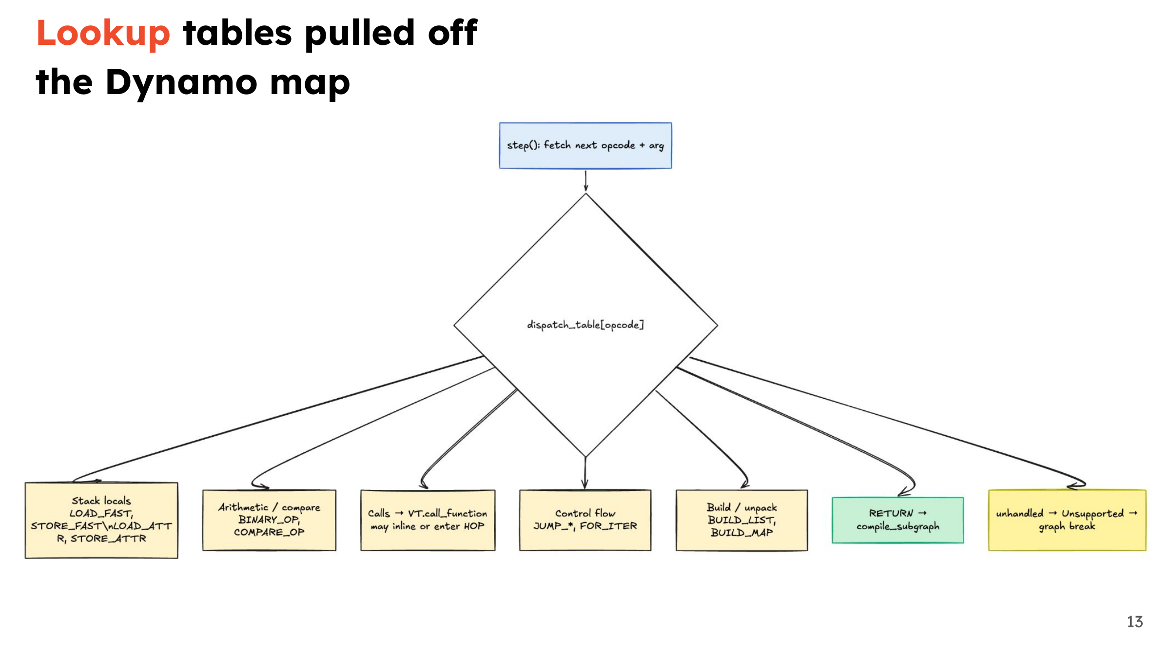
Different bytecodes lead to handlers for stack operations, arithmetic, calls, control flow, and container construction. Those handlers decide what Dynamo can model and what requires a different path. A graph break is one possible outcome when capture cannot continue under the current settings; it isn’t the meaning of every unfamiliar Python instruction.
14. VariableTracker objects
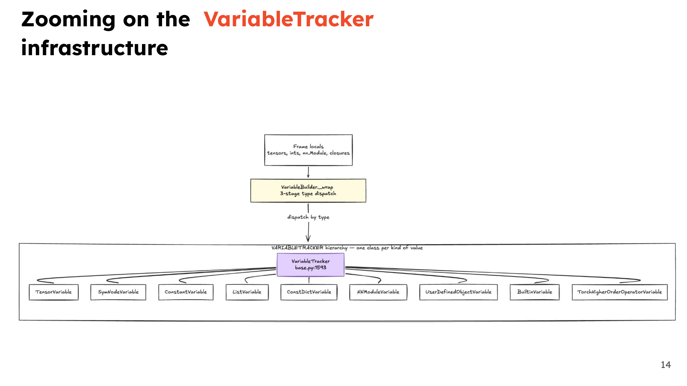
Dynamo wraps values in representations suited to their behavior: tensors, constants, lists, modules, and symbolic integers need different handling. A VariableTracker carries that understanding through the trace. For example, a tensor operation may add an FX node, while reading a known Python constant can be resolved during tracing.
15. The lifecycle of a guard
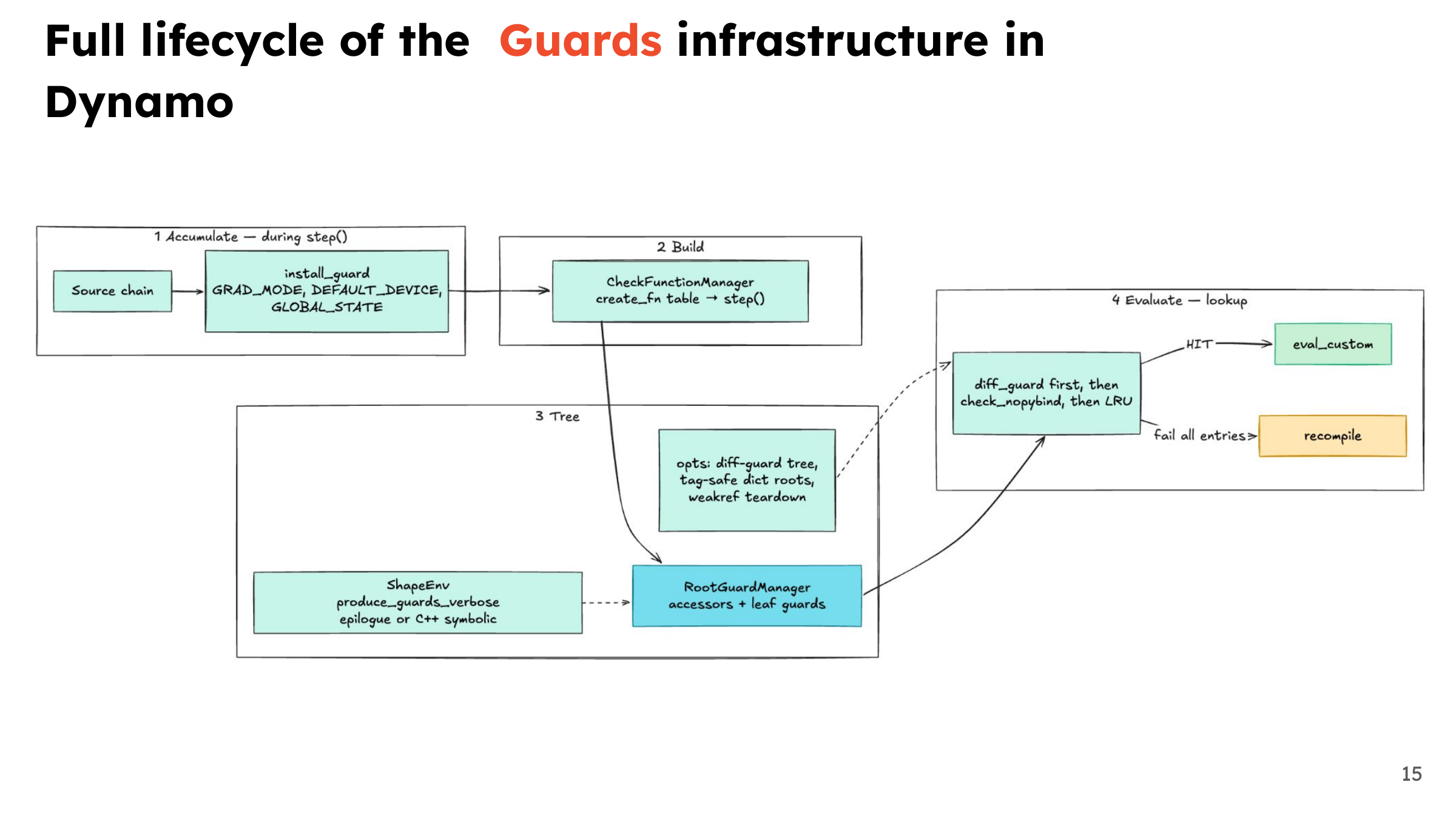
Tracing collects assumptions about inputs and Python state. Guard-building machinery turns them into checks that run when a cached result is considered for reuse. If no cached version matches, Dynamo may retrace or follow a configured fallback path. Guards are part of how specialization remains correct as a Python program changes around it.
16. Graph breaks and recovery
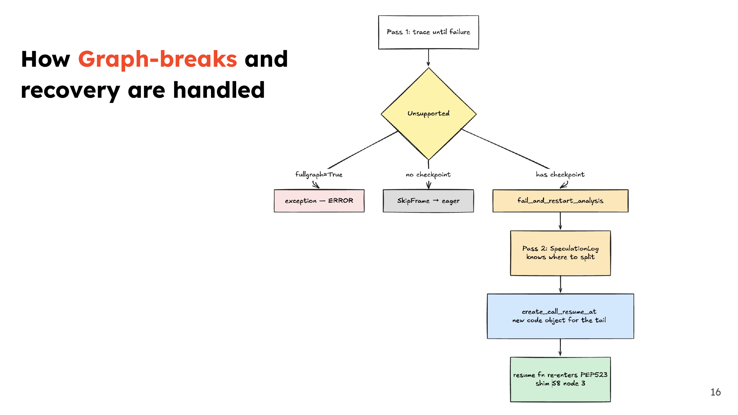
With ordinary partial capture, Dynamo can compile a supported region, execute unsupported work in Python, and resume capture afterward. Continuation bytecode and restored execution state make that possible. With fullgraph=True, a graph break raises an error instead. That setting is useful when you need to know whether the chosen region is fully capturable.
17. The AOTAutograd bridge
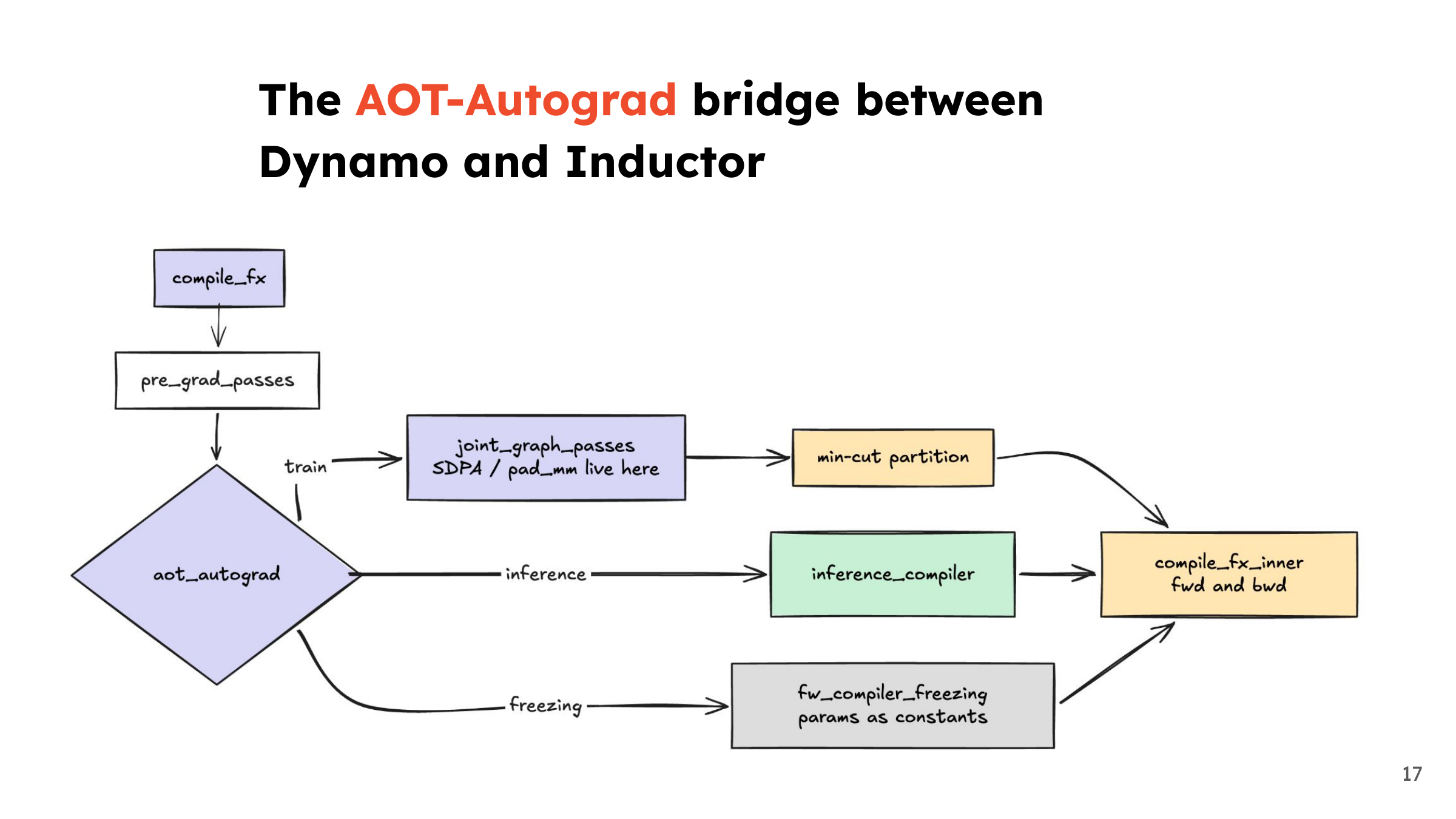
Training requires thinking about forward and backward together: which values should be saved, and which can be recomputed? AOTAutograd prepares graphs that compiler backends can handle, including functionalization and partitioning. Inference takes a different path because no backward graph is required. The name doesn’t mean every torch.compile call becomes an ahead-of-time deployment artifact.
18. Entering Inductor
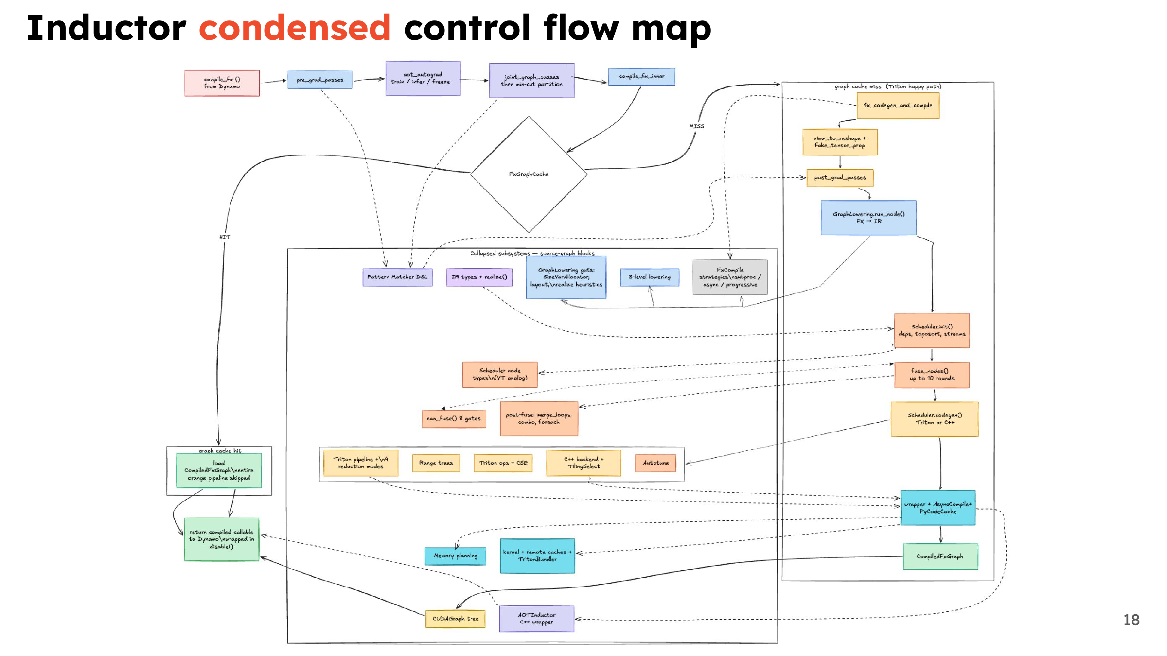
Inductor receives an FX graph and works toward an executable schedule. Graph transformations, lowering, dependency analysis, fusion, code generation, and wrapper construction all fit here. It can emit Triton or C++ code and retain calls to external kernels. A compiled model can therefore contain several kinds of executable work.
19. More than one compiler cache
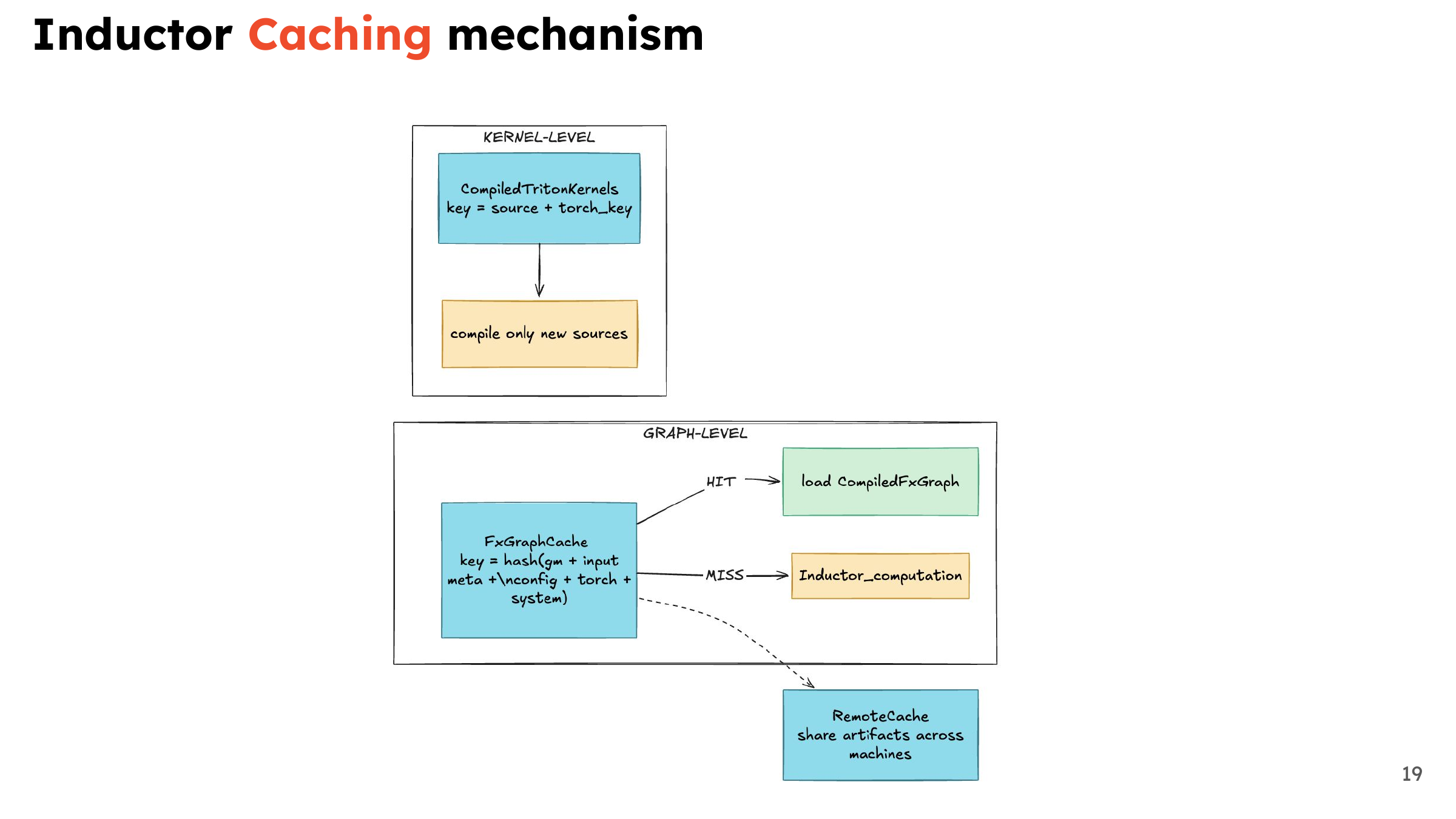
Inductor has caches for graph-level artifacts and lower-level generated code. Their keys need enough information about the computation, configuration, and environment to make reuse valid. A cached kernel can save compilation even when a surrounding graph changes. This is separate from Dynamo deciding whether a Python frame can reuse a previously captured result.
20. Lazy IR and realize()
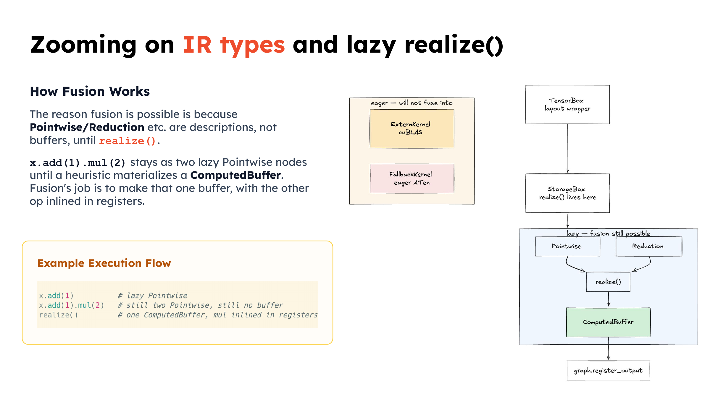
For an expression like x.add(1).mul(2), Inductor can retain a description of computation without immediately committing every intermediate to storage. realize() introduces a materialized buffer representation when needed. That happens while building the compiled program; it doesn’t itself run a GPU kernel. The StorageBox implementation makes this distinction concrete.
21. GraphLowering builds the next representation
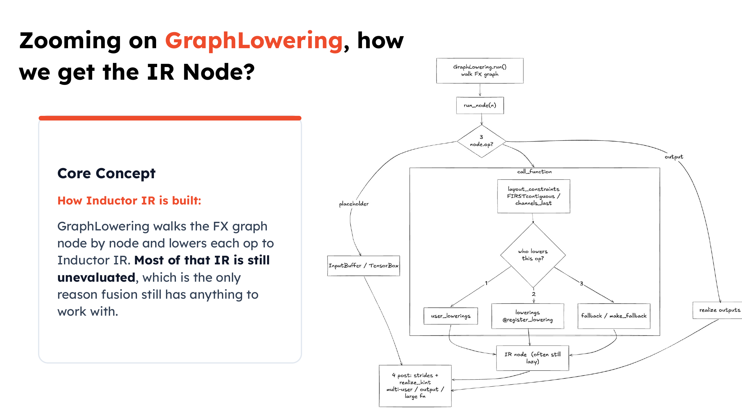
GraphLowering walks the FX graph and translates operations into Inductor’s representation using registered lowerings or supported fallback paths. Shapes, layouts, and how values are produced become more explicit. Retaining computation in a form that can still be combined gives later scheduling and fusion passes something useful to work with.
22. Building the scheduler’s dependency graph
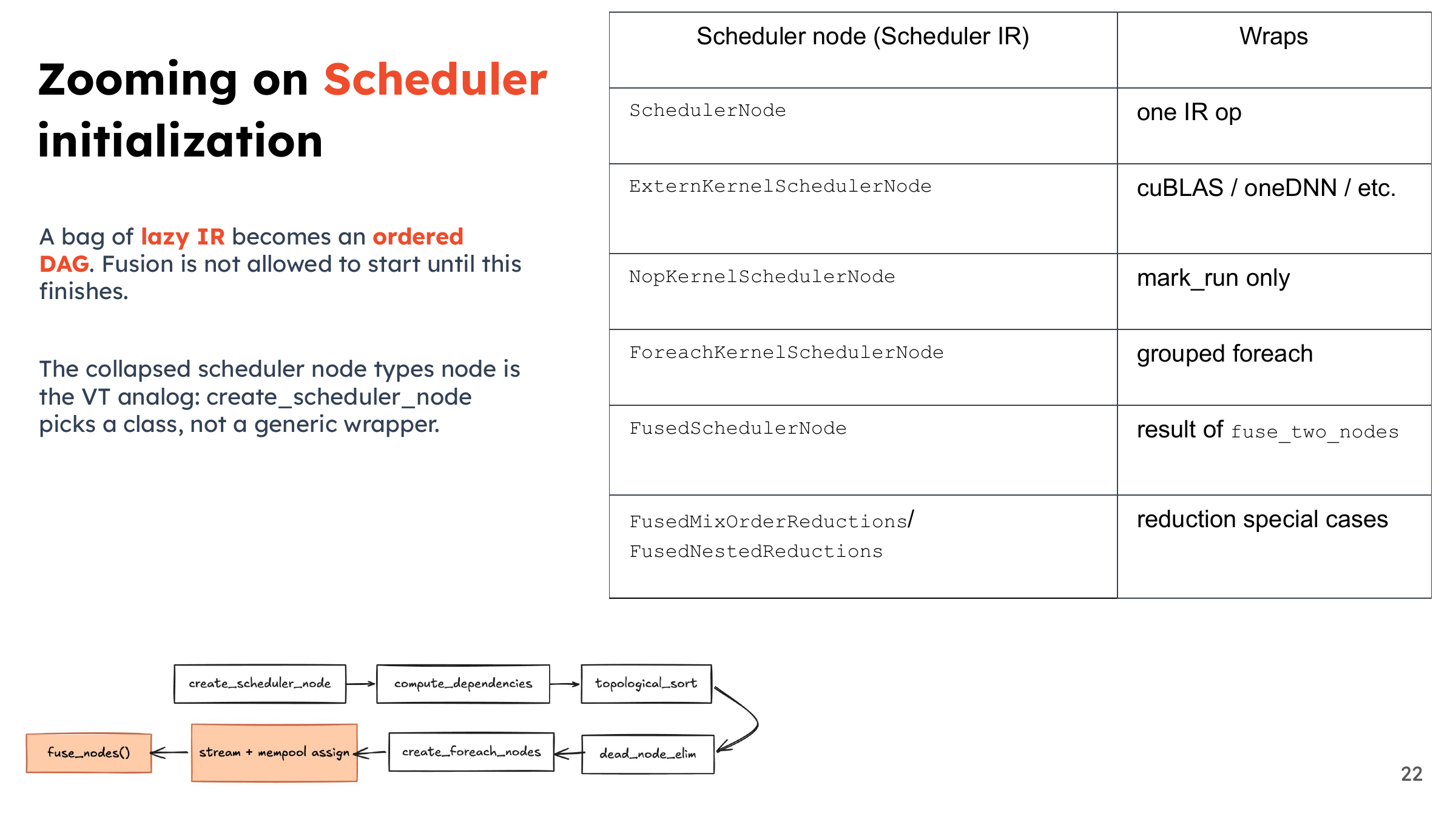
The scheduler needs to know which operations read and write which buffers before it can reorder or combine them. It creates nodes for generated work, external kernels, and other execution categories, then establishes dependencies. An external library call has different scheduling and code-generation constraints from a pointwise expression that Inductor controls directly.
23. When can two operations fuse?
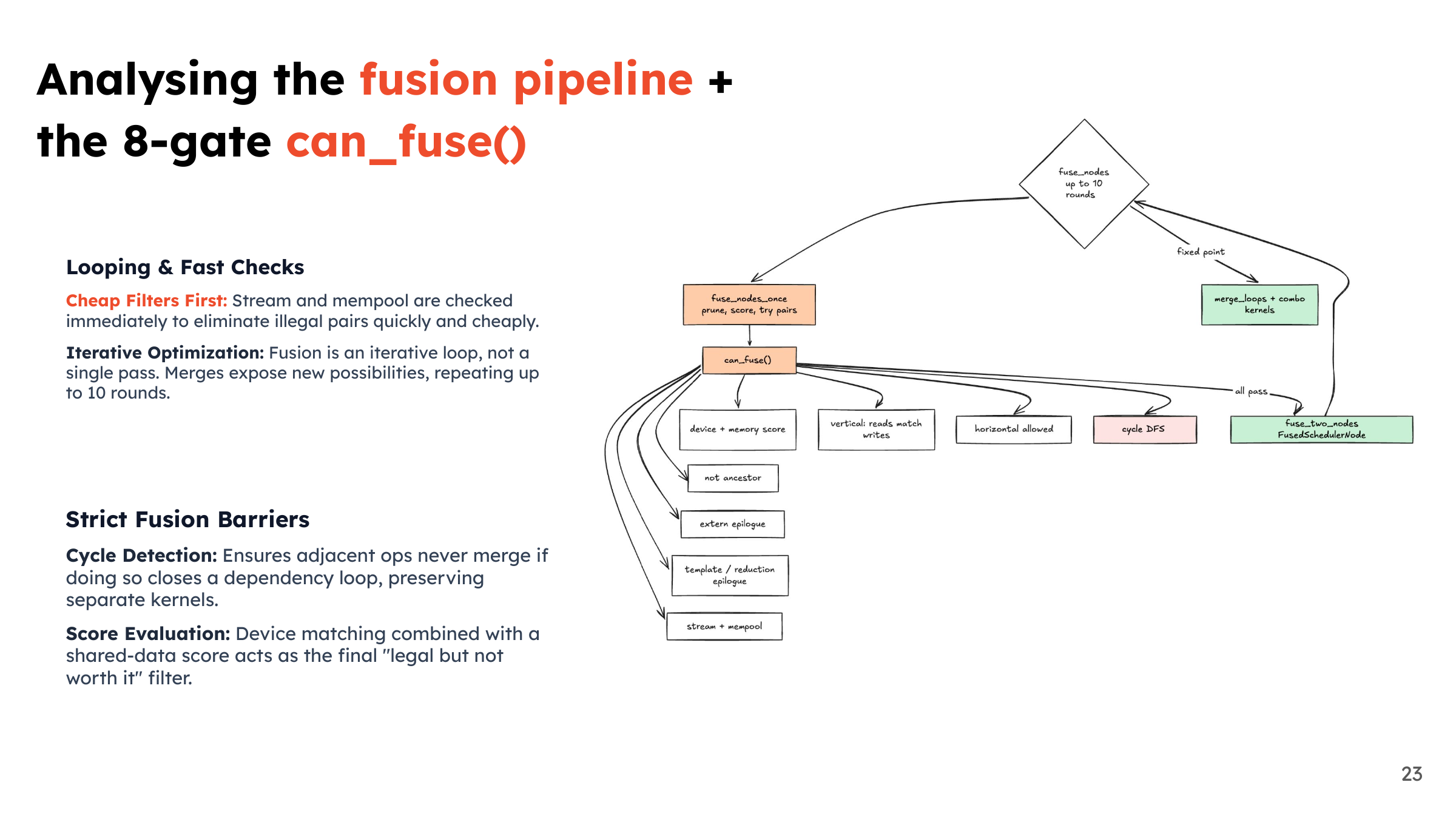
Fusion needs both a legality check and a reason to expect a benefit. Dependencies, devices, layouts, and backend restrictions can prevent a merge; profitability checks can reject one that is technically possible. The exact gates and iteration limits evolve. The useful idea in scheduler.py is that fewer kernels alone isn’t a complete performance model.
24. Choosing the code-generation path
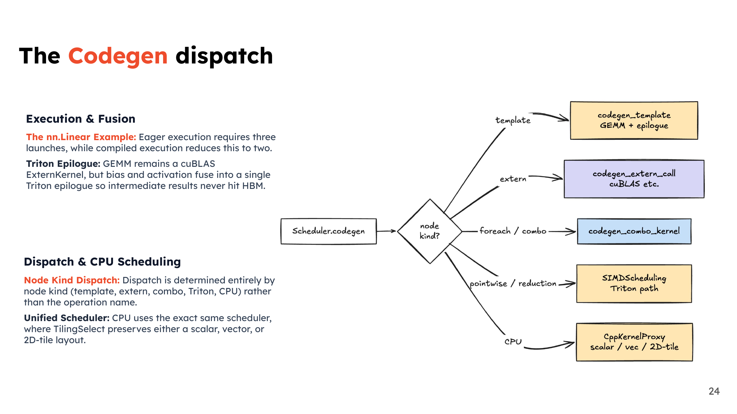
The kind of scheduled work determines whether Inductor emits a template, an external call, Triton, or CPU code. A matrix multiply followed by bias and activation may use a library GEMM plus a fused pointwise kernel. In that case the GEMM result still crosses the kernel boundary; only intermediates inside the fused region avoid separate materialization. Launch counts depend on the chosen implementation.
25. Wrappers, memory, and compilation jobs
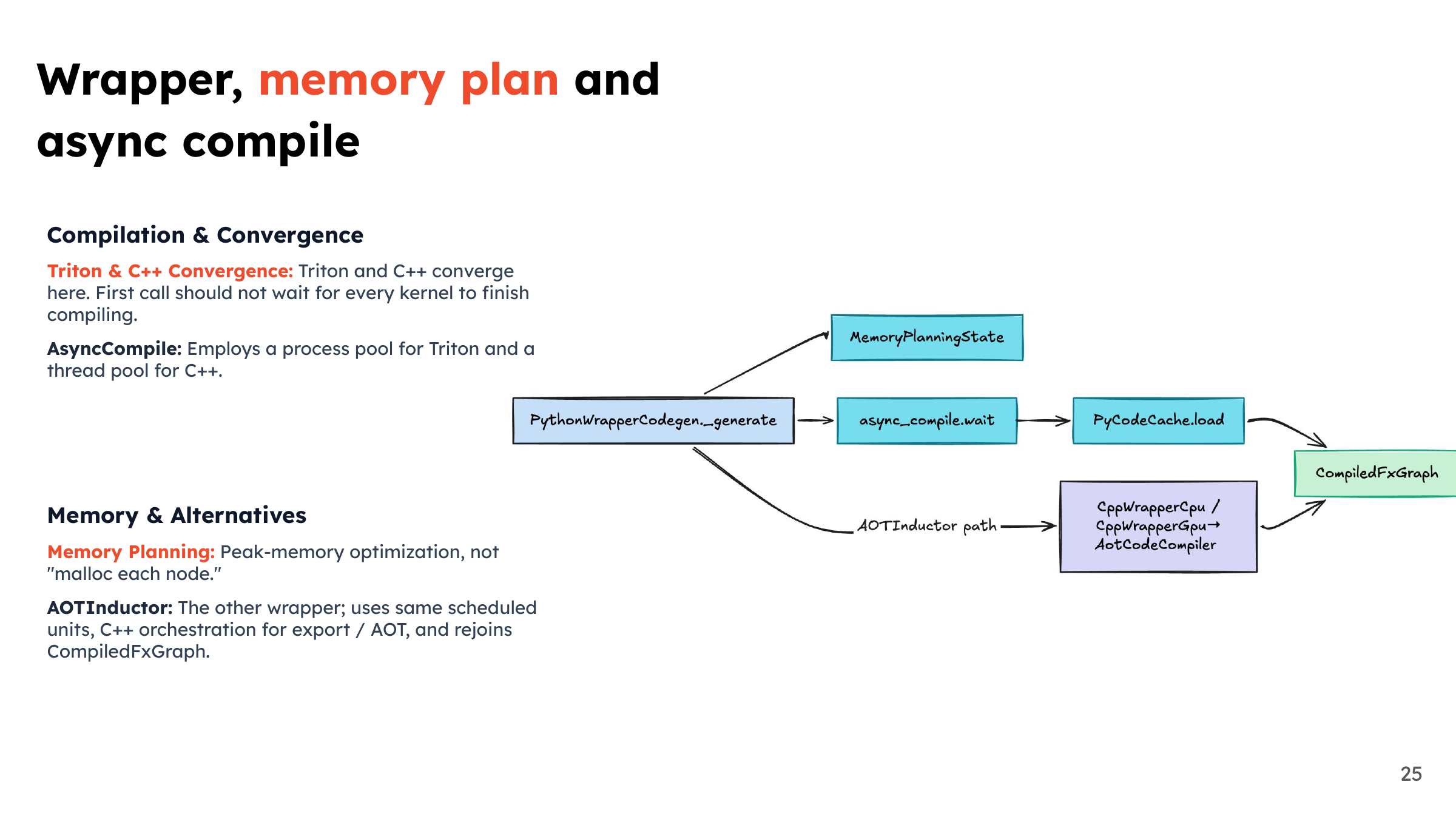
Generated kernels need a wrapper that arranges inputs, manages buffers, and invokes work in the right order. Memory planning can reuse storage whose previous contents are no longer needed. Kernel compilation jobs can overlap, but execution still has to wait for the code it needs to become ready. Asynchronous compilation doesn’t remove that dependency.
26. CUDA graph trees
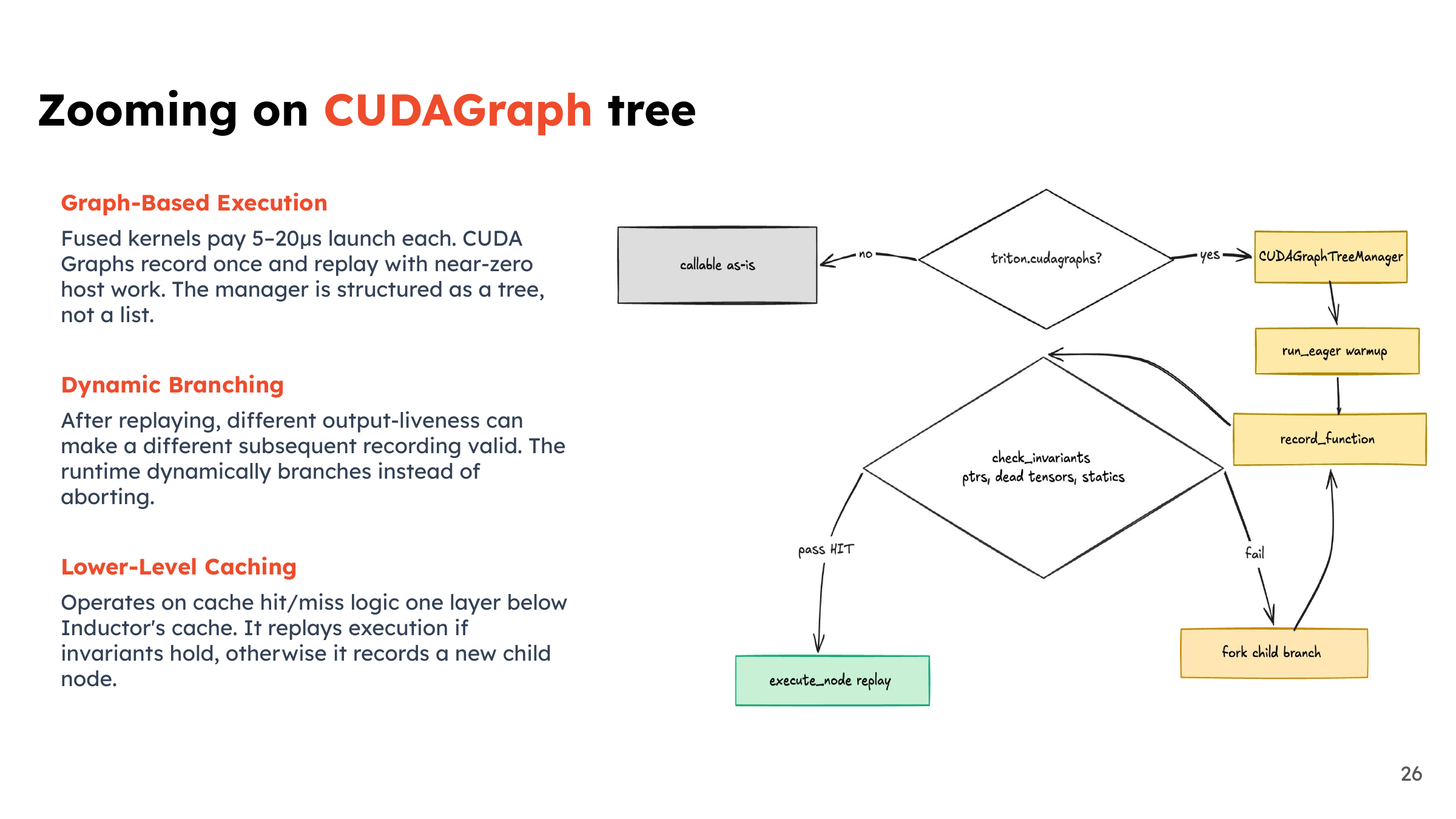
CUDA graphs record a compatible sequence of device work so later calls can replay it with less CPU dispatch. Inductor’s tree machinery also considers execution paths and tensor lifetimes when deciding whether a recording is reusable. Replay still has overhead and validity conditions. It is another runtime optimization layered on top of generated code.
27. Autotuning
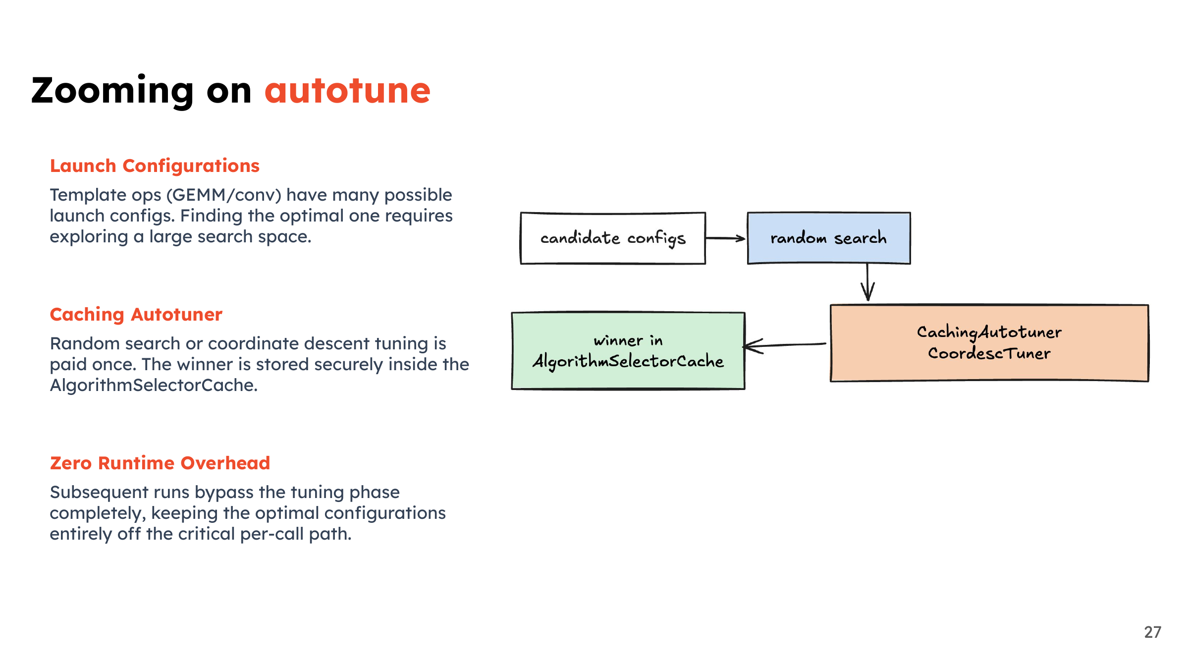
A matrix multiplication or reduction can have several plausible implementations or launch configurations. Autotuning measures candidates and caches a choice for the relevant workload. Kernel-level launch tuning and graph-level algorithm selection are related but distinct pieces of this process. More tuning can improve steady-state execution while making startup more expensive.
28. Putting the stages back together
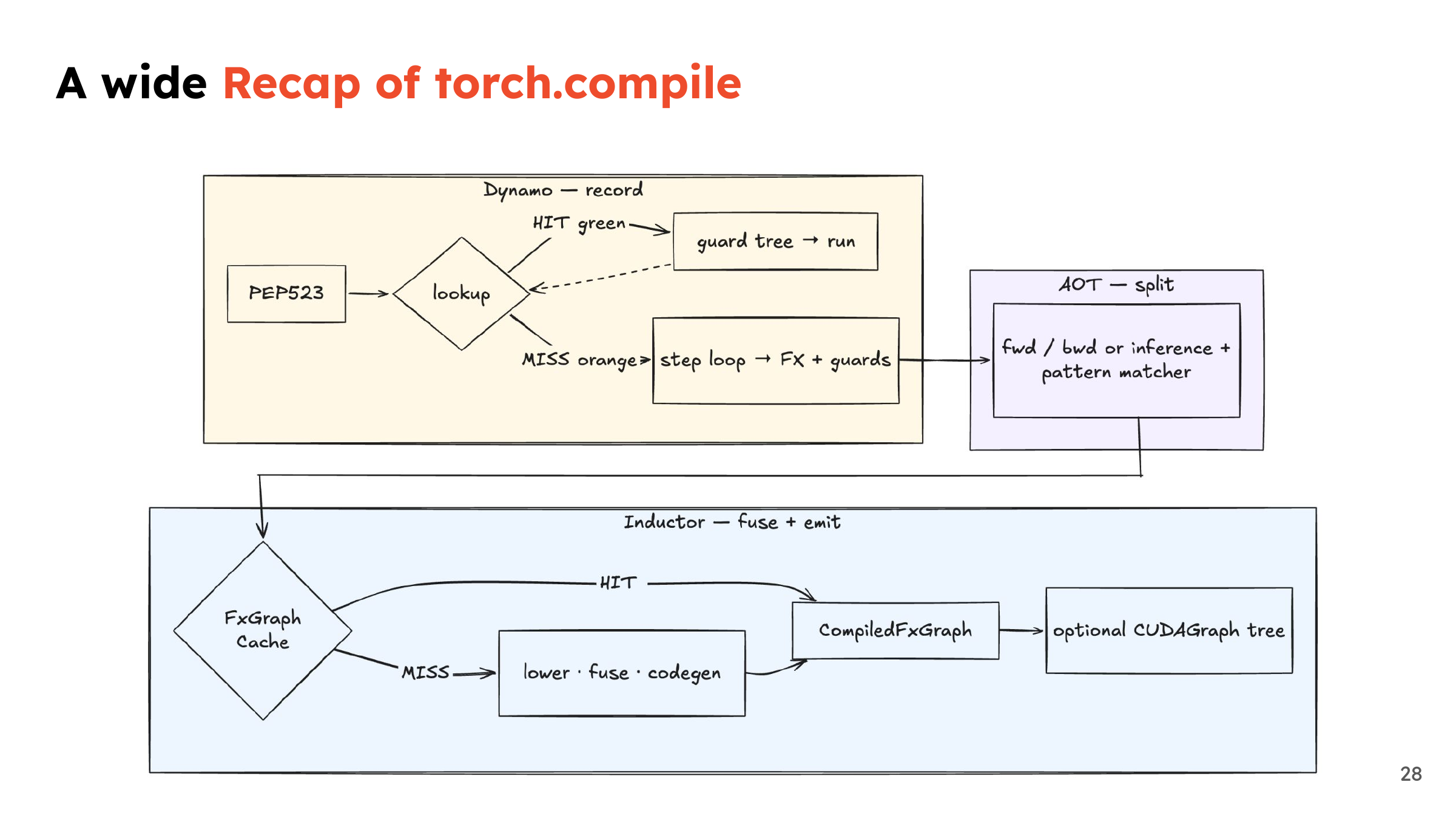
The final picture connects capture, transformation, lowering, and reuse. When debugging, I would first identify which stage is doing unexpected work: a guard miss, a graph break, repeated kernel compilation, or a new CUDA graph capture are different events. That distinction helps turn a vague slow-compile problem into something you can inspect.
29. References and the larger drawing
The diagrams are meant to be read alongside the PyTorch source. The slide also links to my full Excalidraw illustration, where the connections are easier to explore. Start with one function and follow its path through the map instead of trying to memorize every box.
30. Thanks for following along

I hope this makes the compiler feel a little less opaque. A useful next experiment is to run the same small function twice, then change an input shape and inspect what gets reused. Once that behavior makes sense, the larger graphs become much easier to reason about.