Calling torch.compile takes one line. Understanding how it gets hold of your Python code takes a little more work. In this talk, I followed that path from CPython’s frame evaluator to the FX graph that Dynamo hands to a compiler backend.
These are the slides from my March meetup talk, with a short explanation for each one. Click any slide to read the diagram at full size. The bytecode examples are simplified; instruction names and frame layouts depend on the Python version.
1. From Python to an FX graph
The question I wanted to answer was fairly small: how does a regular Python function become a graph? Before worrying about generated CUDA or Triton code, we need to understand how Dynamo captures the computation in the first place. This talk stays mostly on that side of the compiler.
2. What is TorchDynamo?
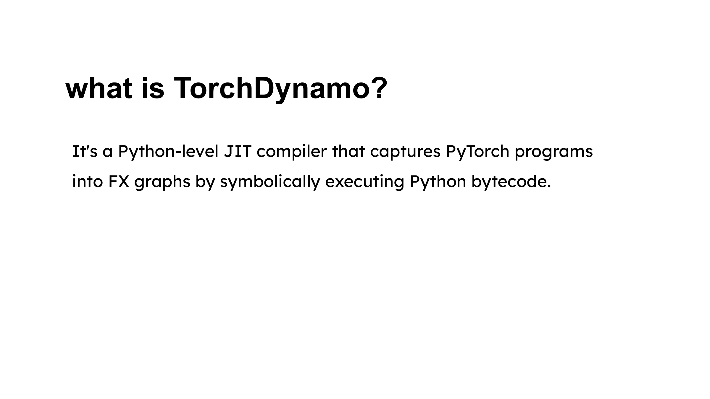
Dynamo is the part of torch.compile that watches Python execution and captures tensor operations. It symbolically interprets bytecode, builds an FX graph, and records the assumptions under which that graph is valid. The output also includes Python bytecode for the work around the graph; a Python function doesn’t have to become one giant tensor operation.
3. How does it get into Python execution?
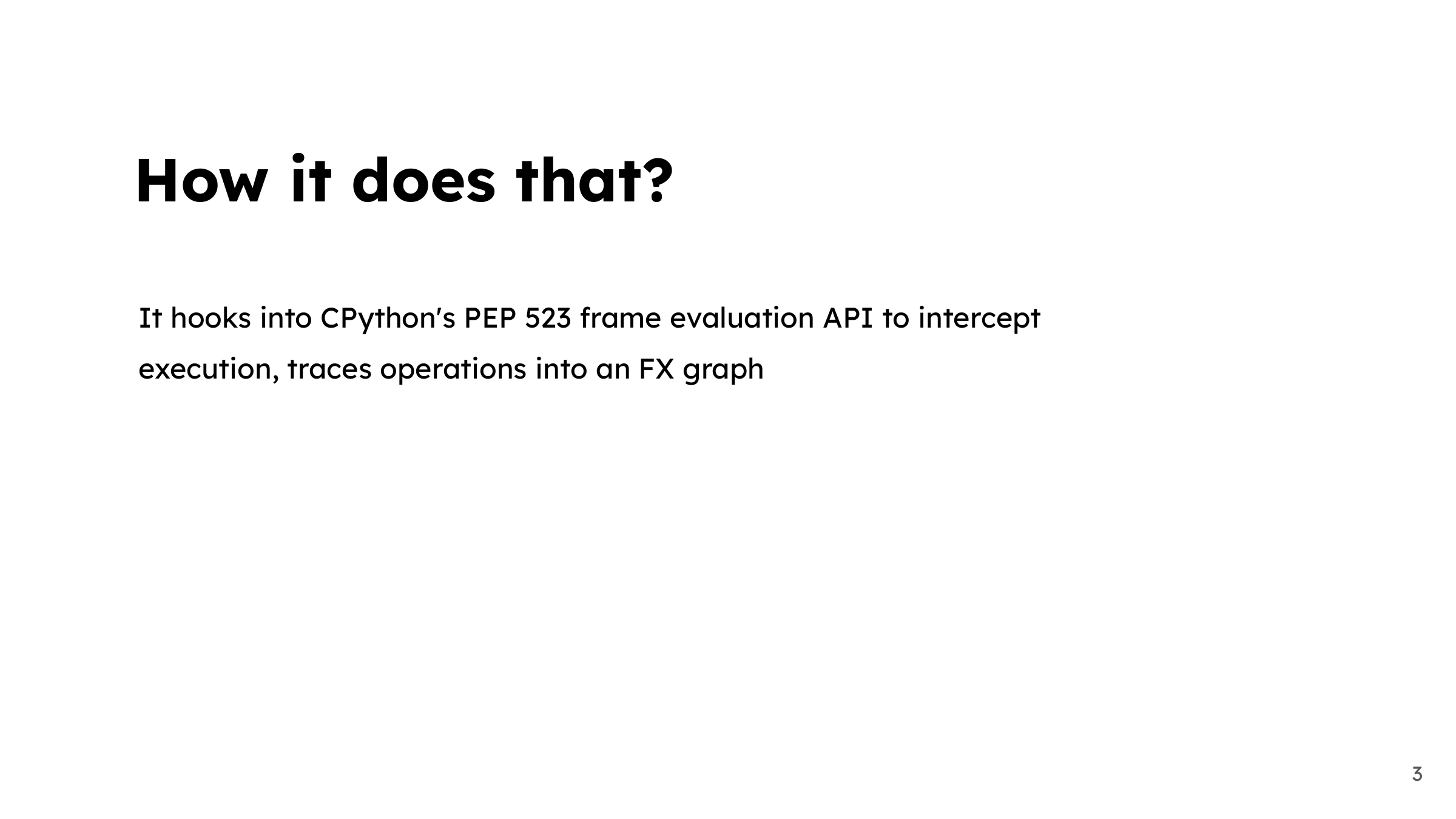
CPython provides a frame evaluation hook through PEP 523. Dynamo uses that hook to intercept a frame before the normal evaluator executes it. That gives it access to the code and runtime state needed for tracing, without requiring you to rewrite the function in a separate language.
4. A few CPython prerequisites
Three things help here: a code object describes what to execute, a frame holds the state of a particular execution, and the evaluation loop walks through the instructions. Keeping those separate makes the rest of the diagrams much easier to follow. The function’s instructions and the values passed into it are different pieces of the story.
5. Source code becomes bytecode
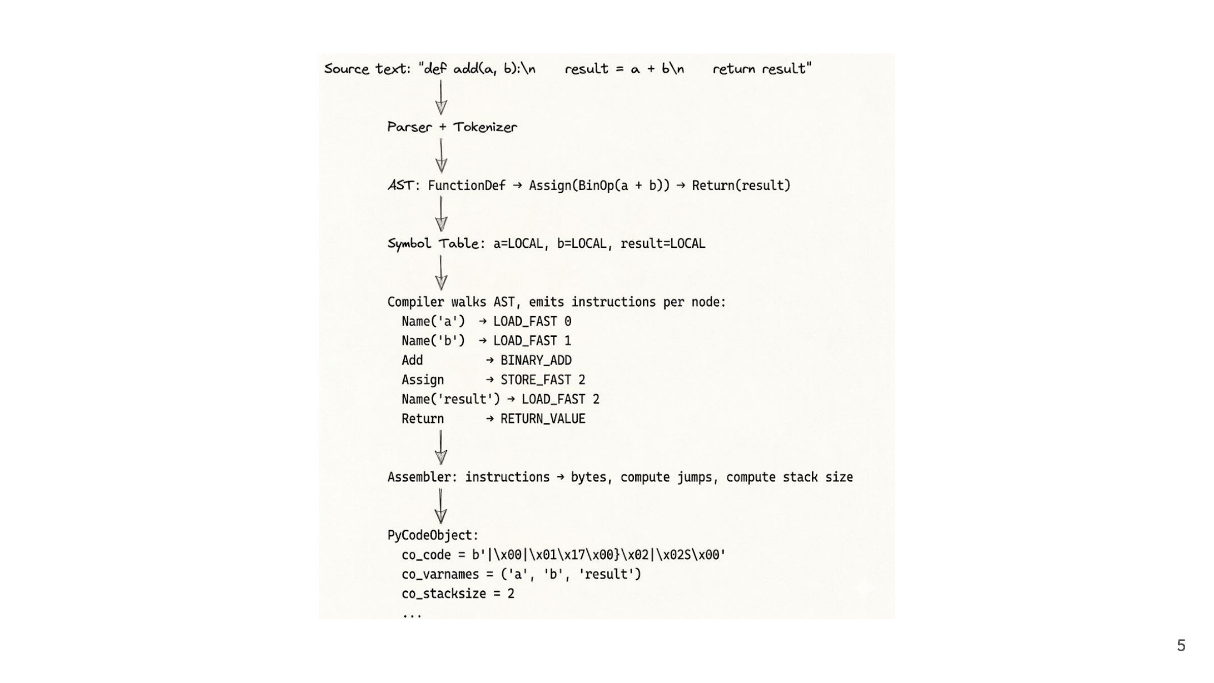
Take a tiny function that adds two arguments. CPython parses its source, builds an AST, resolves names, and produces a code object containing bytecode and related metadata. Dynamo starts from those instructions. It doesn’t need to recover your original source text to discover that the function loads two values, adds them, and returns the result.
6. A frame makes the instructions executable
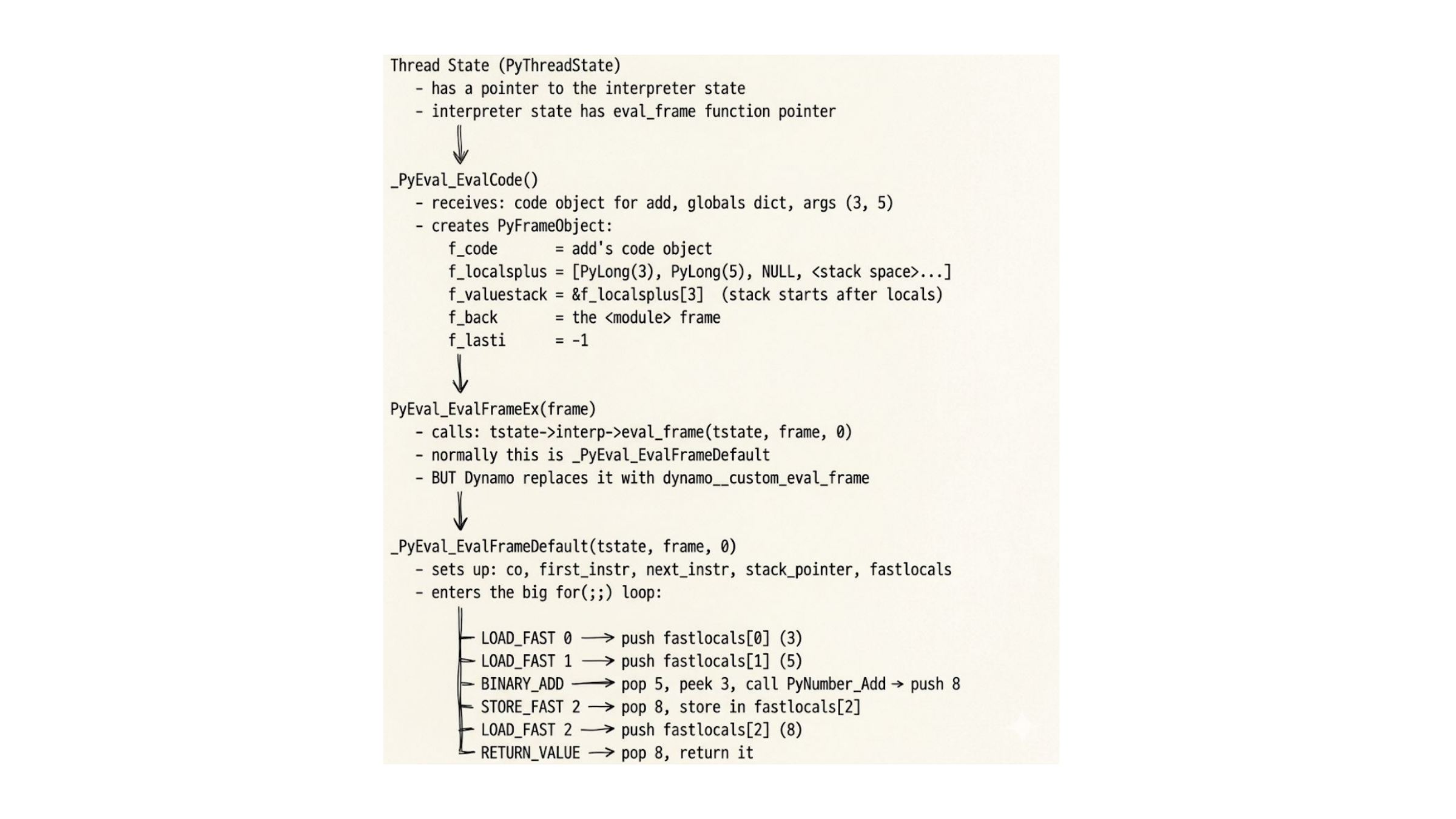
The same code object can run with many different inputs. A frame connects it to the current locals, globals, and evaluation stack. The diagram follows a simple addition through that stack: load the arguments, perform the operation, store the result, and return it. Dynamo will build a symbolic version of this process.
7. Two entry points meet
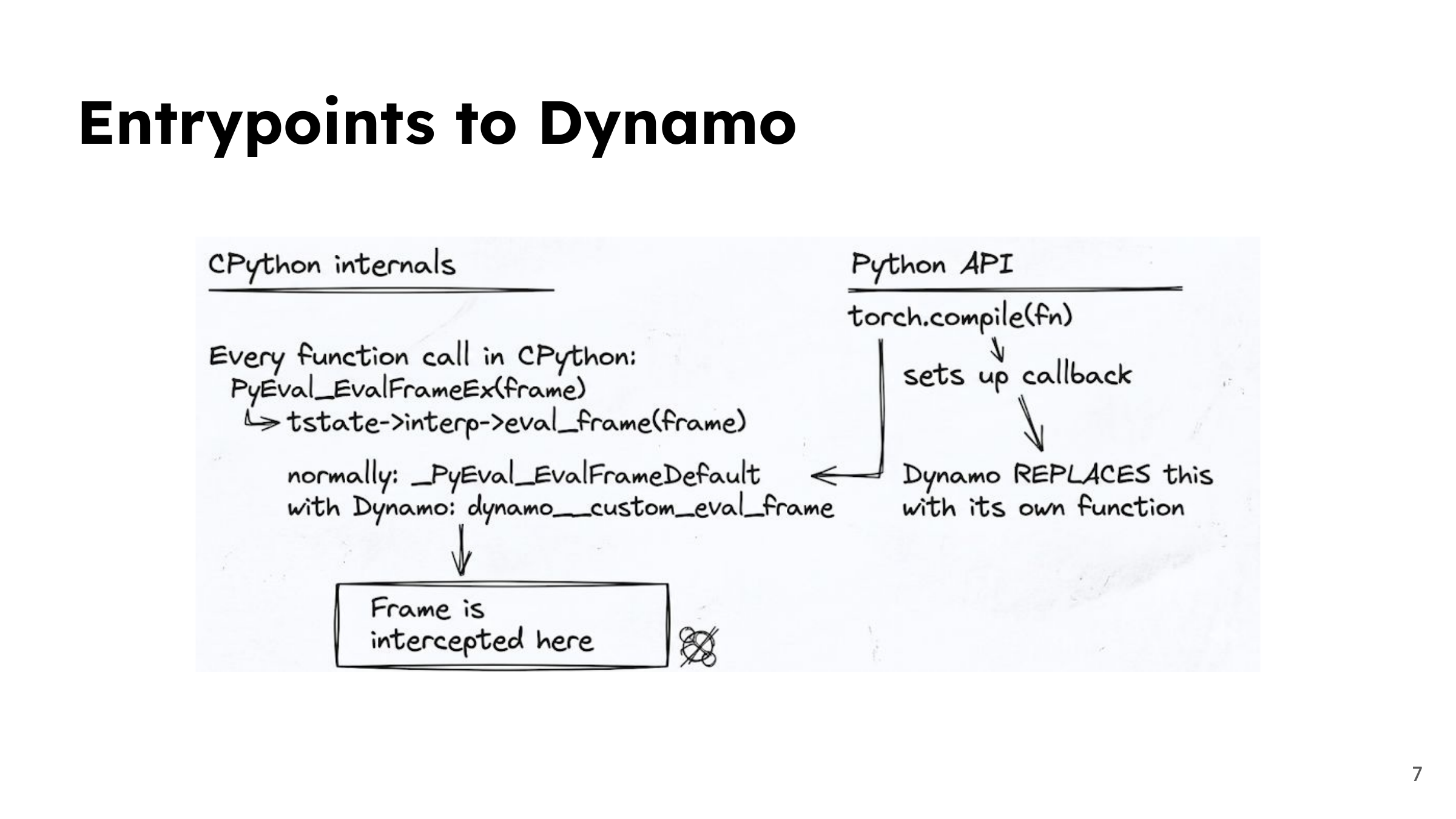
There are two paths to keep in mind. On the Python side, torch.compile(fn) prepares a wrapper and a tracing callback. On the CPython side, the frame evaluation hook decides what to do when execution reaches a frame. The wrapper activates the context in which those two paths can meet.
8. Let’s use a small example
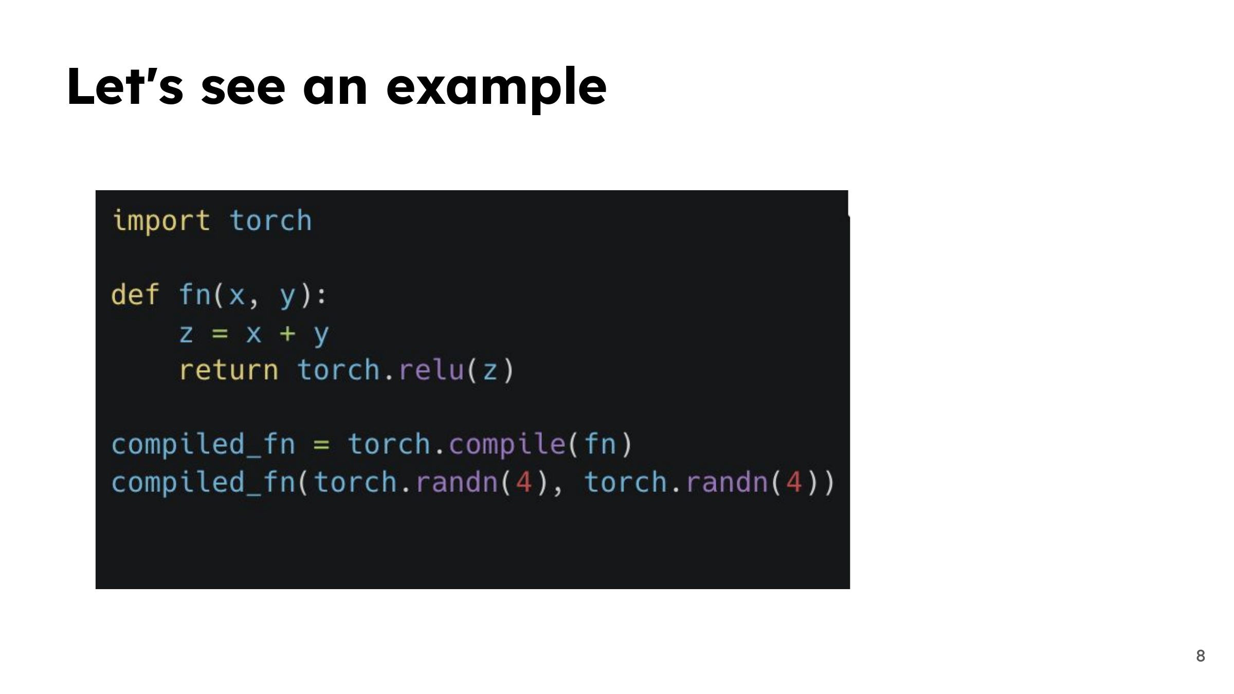
Our function computes z = x + y, then returns torch.relu(z). There are only two tensor operations, which makes it easy to follow each one into the graph. Calling torch.compile(fn) prepares the callable; the first invocation with actual inputs is where tracing normally starts.
9. Reading the bytecode
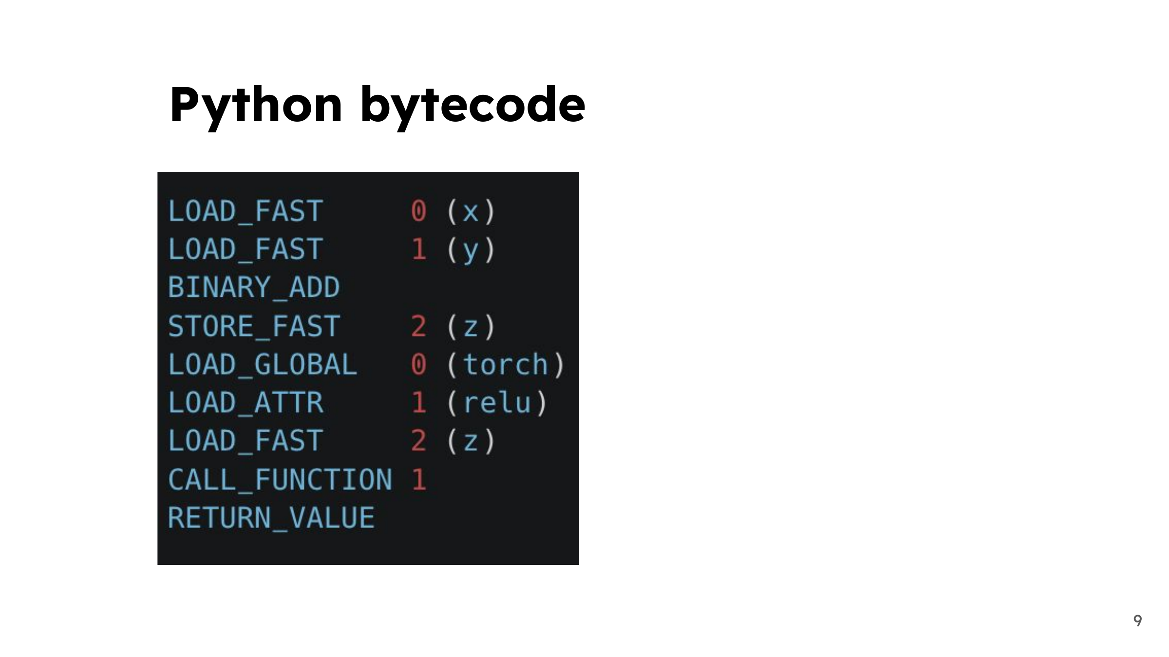
The instructions load x and y, add them, store z, look up torch.relu, and call it. The operand stack connects these steps. If your Python version shows BINARY_OP or different call instructions instead of the names in the slide, that’s expected. The useful part is the movement of values through the stack.
10. What the frame contains
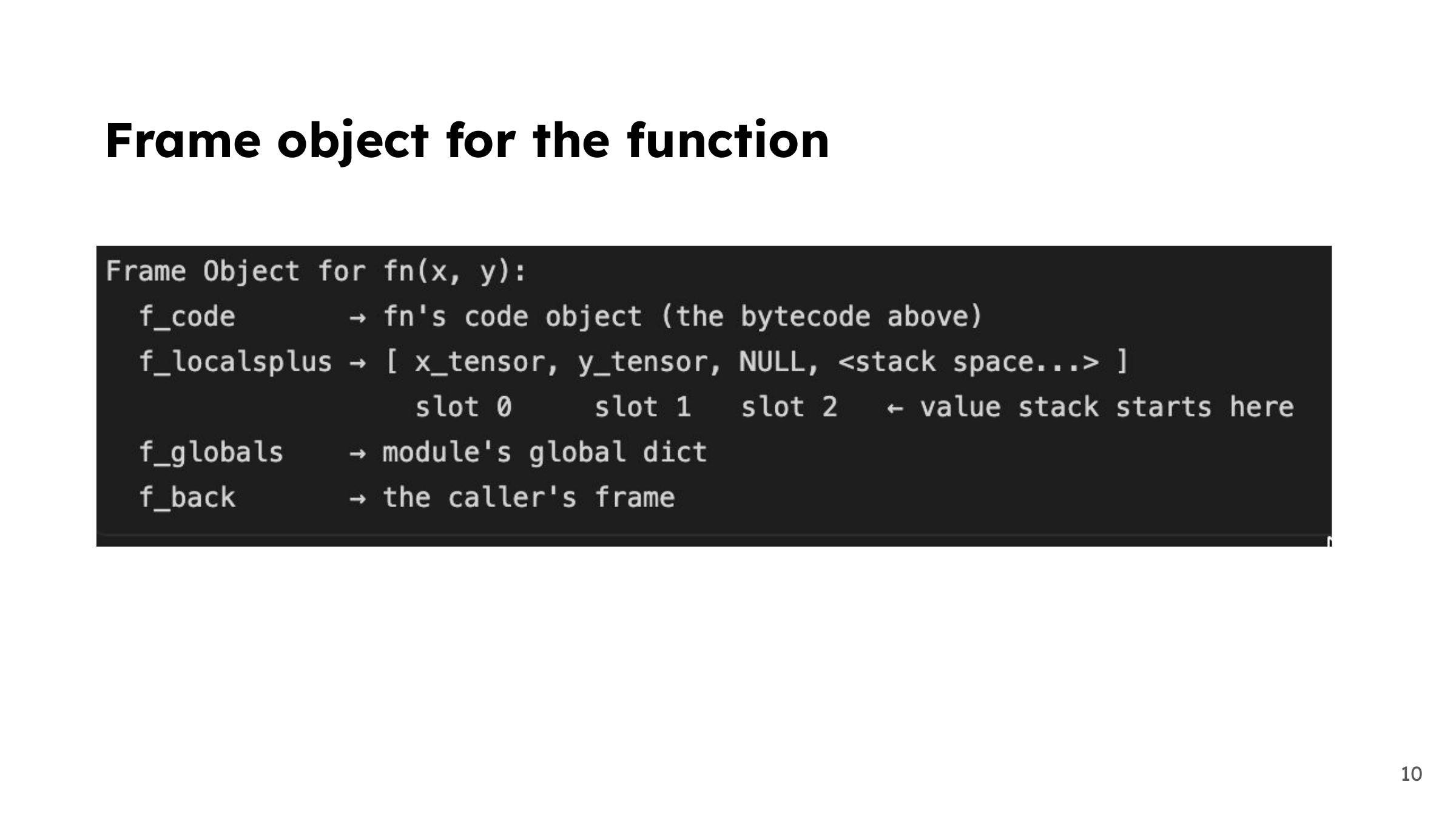
At the function call, the frame has the code object, references to the input tensors, and access to globals such as torch. That is enough context for Dynamo to start reasoning about the function. The exact C structure has changed across CPython releases, so I use this diagram as a map of responsibilities rather than a fixed memory layout.
11. Installing the hook
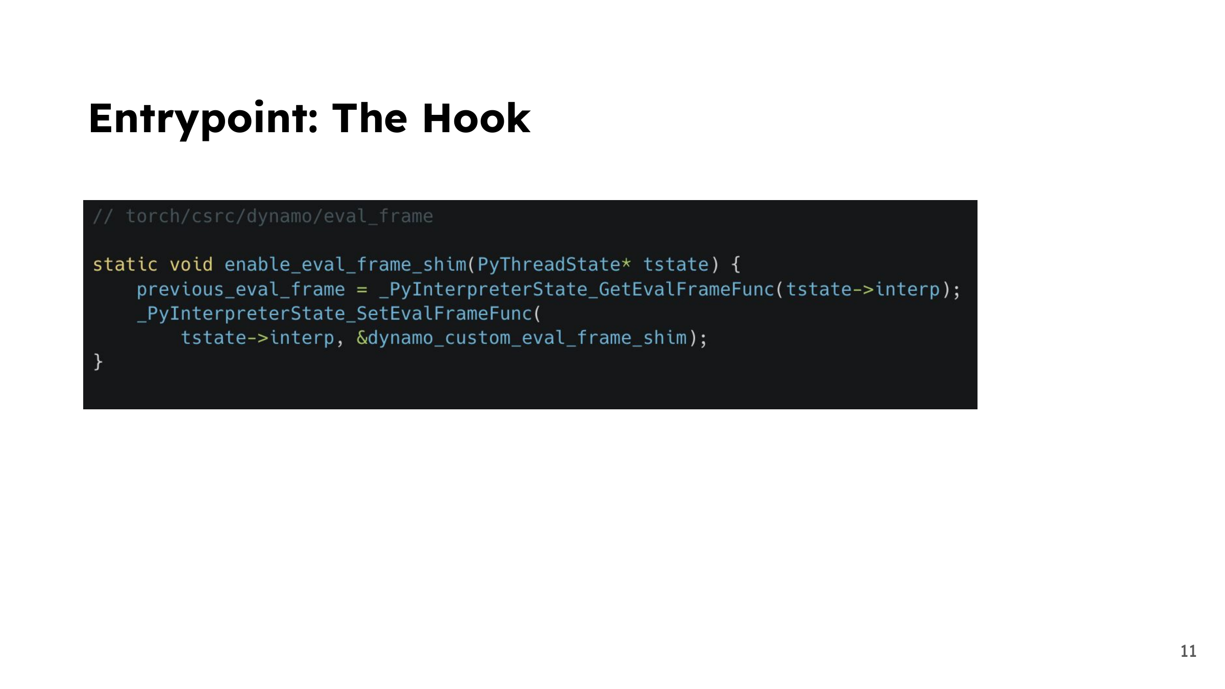
The C/C++ side connects CPython’s evaluator to Dynamo’s custom frame evaluation path. This is the bridge between Python’s execution machinery and the compiler callback. The implementation lives in PyTorch’s eval_frame.c; the small snippet here highlights the hook installation rather than all the surrounding checks.
12. The Python setup path
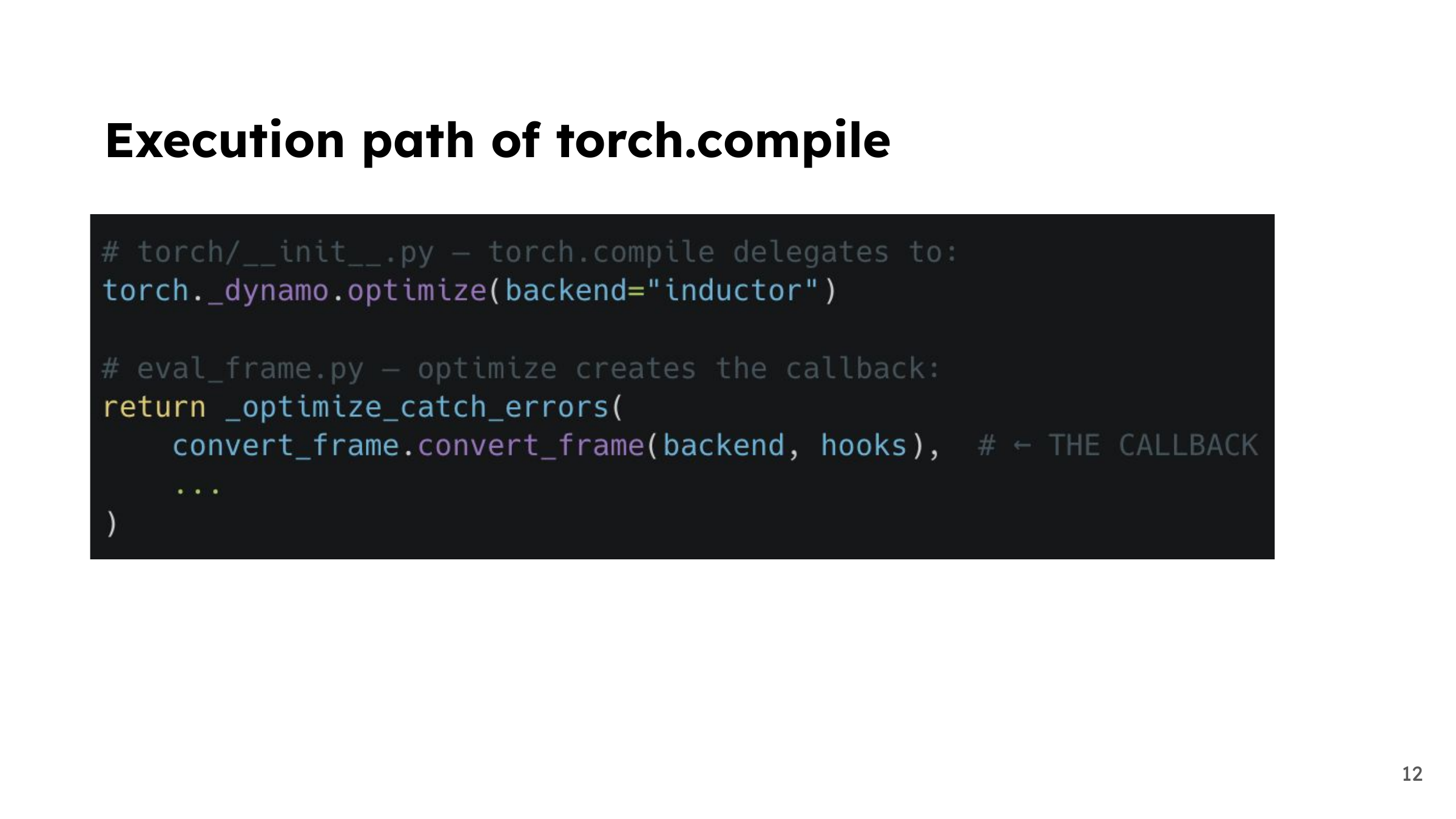
From the public API, execution reaches Dynamo’s optimization machinery, resolves the backend, and prepares a frame conversion callback. With the usual Inductor backend, the graph will eventually travel further down the compiler stack. At this point, though, we’re setting up how a frame will be traced, not generating GPU kernels yet.
13. Where the paths combine
Now we can connect the setup to execution. The compiled wrapper has arranged the callback, and calling the function creates a frame. When the evaluator intercepts that frame, it can check for a reusable compiled result or hand the frame to the Python tracing callback.
14. Following the first call
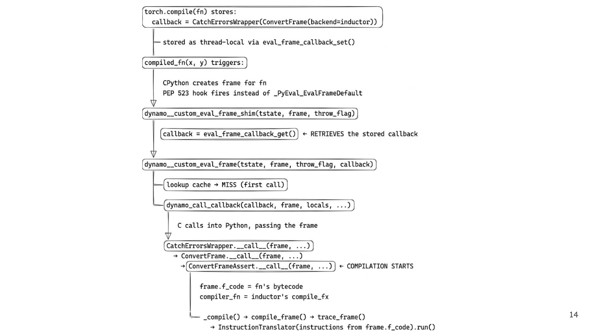
Read this diagram from top to bottom: activate the callback, intercept the frame, check the cache, and enter frame conversion on a miss. That conversion eventually creates an InstructionTranslator. The C/C++ path handles entry and dispatch; the Python translator does the detailed work of interpreting the function symbolically.
15. Disassemble, trace, reassemble
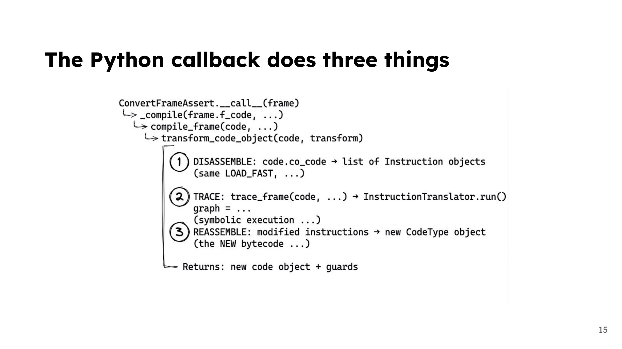
The callback turns bytecode into instruction objects, traces those instructions, and constructs replacement bytecode that can call the captured computation. It also produces guards. Those checks are necessary because the result was built using facts about this particular execution, such as tensor metadata and the Python objects encountered along the way.
16. The symbolic instruction loop
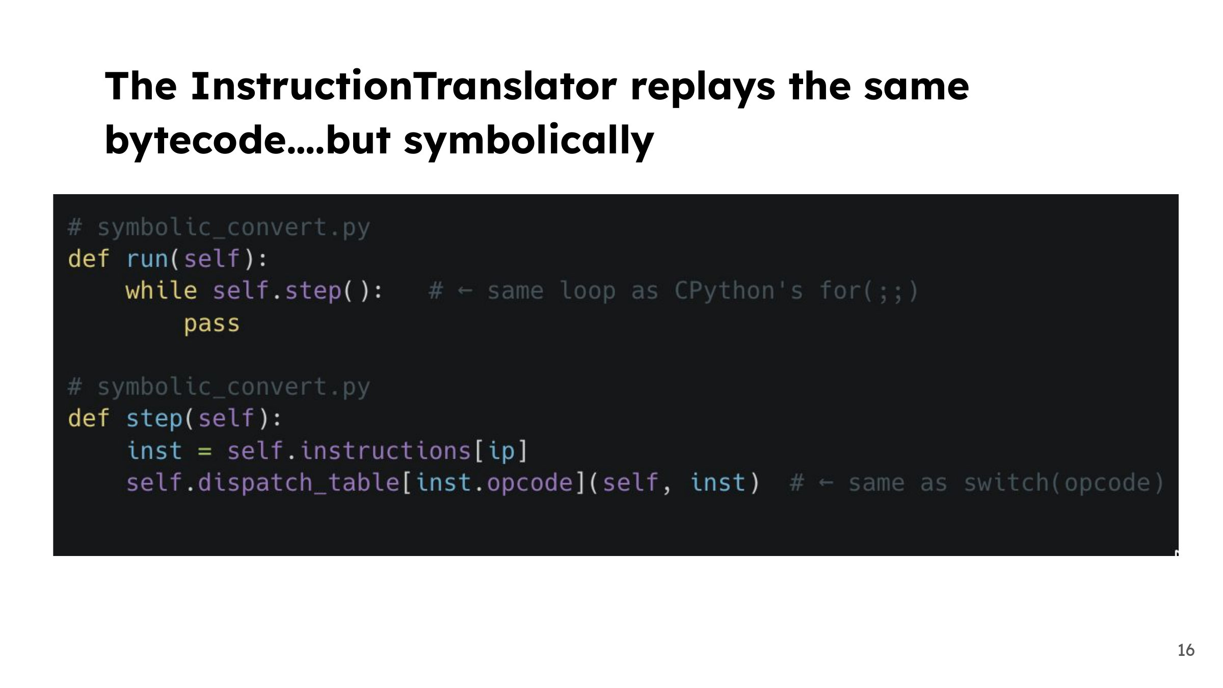
InstructionTranslator repeatedly calls step(), which fetches an instruction and dispatches to its handler. This looks familiar if you’ve seen an interpreter loop. The difference is in the values it manipulates: Dynamo tracks symbolic representations and graph references while preserving the behavior of the program. You can follow the loop in symbolic_convert.py.
17. Real execution and symbolic execution
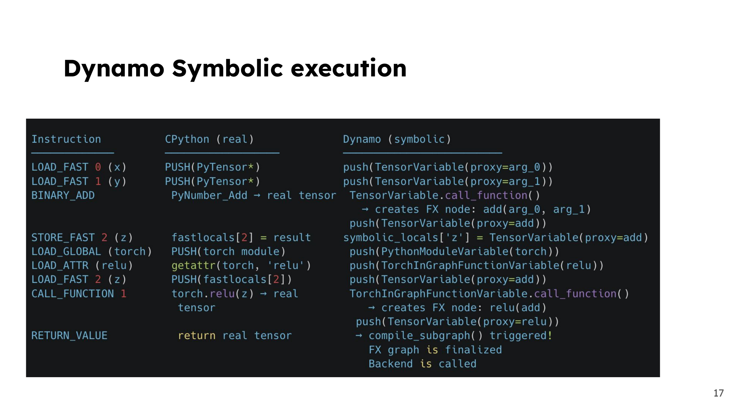
For x + y, normal execution computes a tensor result. Dynamo can instead connect symbolic tensor inputs to an addition node, then connect that node to relu. The symbolic stack still follows the bytecode’s order. The final graph describes the tensor computation that a backend will execute later.
18. The three layers of tracing
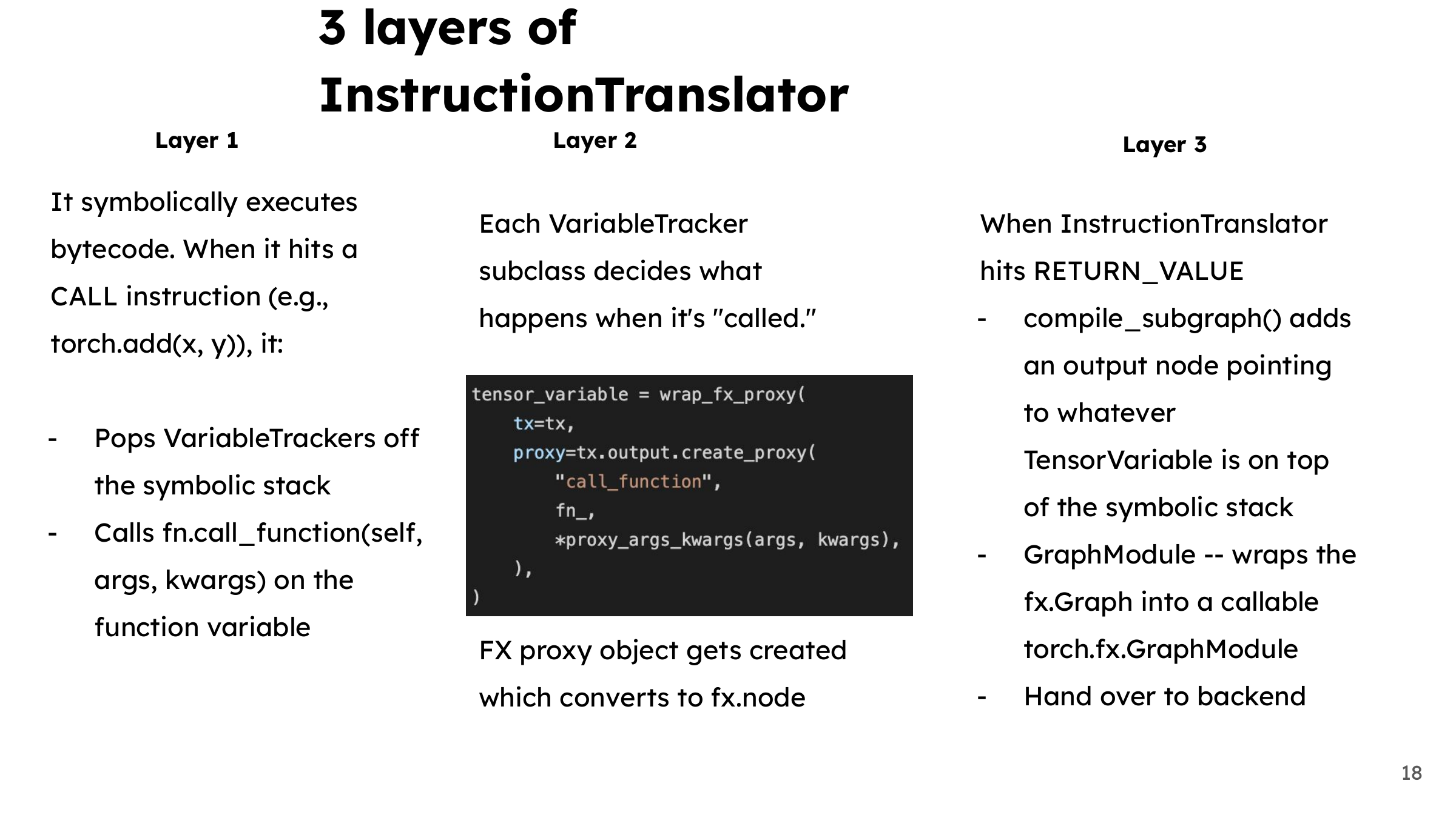
The instruction handler manages the stack, a VariableTracker describes how a particular kind of value behaves, and FX proxies connect tensor operations to graph nodes. When the function returns, Dynamo finalizes the graph outputs and invokes the backend. These layers explain why handling a Python list and handling a tensor call take different paths through the same translator.
19. What happens after capture?
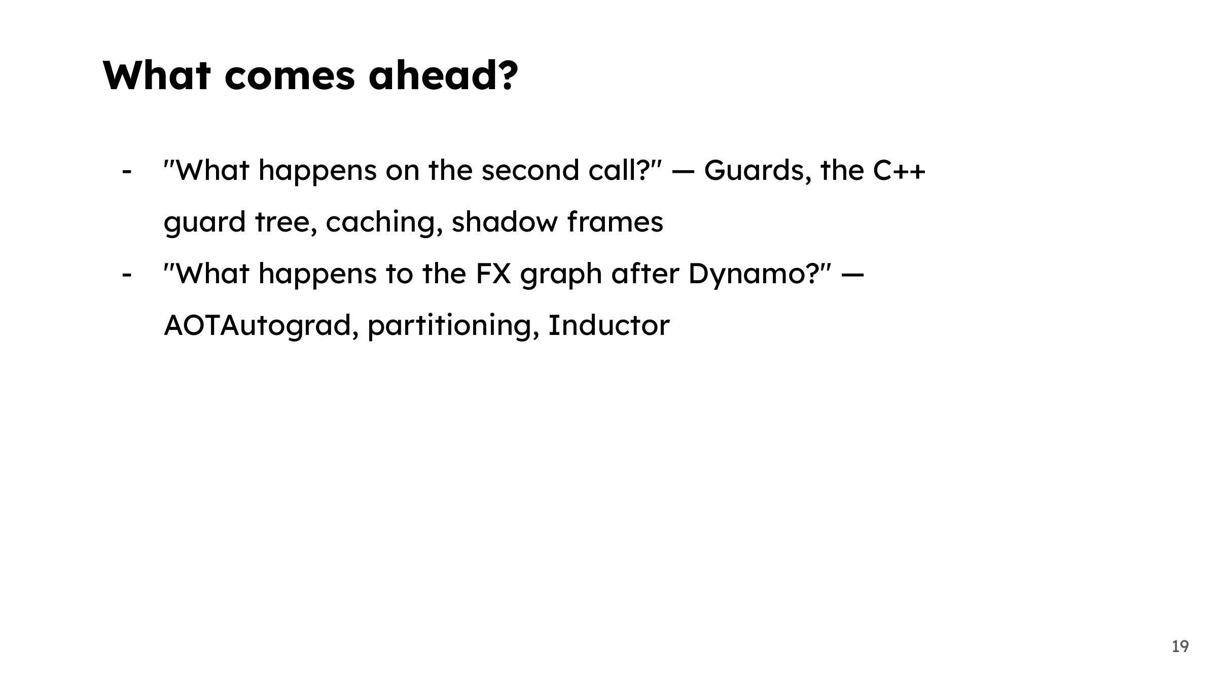
Two questions naturally follow. On the next call, how does Dynamo know whether it can reuse the graph? And once capture finishes, how does that graph become executable code? Guards and caching answer the first; AOTAutograd and Inductor answer much of the second. I cover those in the end-to-end torch.compile walkthrough.
20. Try tracing one tiny function
Thanks for following the talk. If you’re reading Dynamo for the first time, start with a function as small as our addition and ReLU example. Follow its bytecode, symbolic stack, and FX nodes together. That gives the larger compiler diagrams something concrete to attach to.